분류기의 성능을 평가하기 위해 간단히 accuracy (정확도)만을 사용할 수도 있지만 더 정확하게 평가하기 위해서 confusion matrix (오차 행렬) 를 조사하는 것이 필수적입니다.
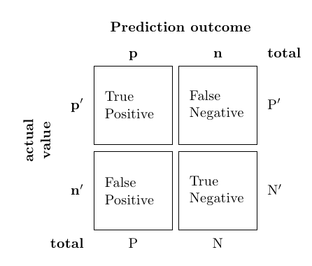
1. Accuracy = $\frac{\text{TP + TN}}{\text{All}}$
2. Precision = $\frac{\text{TP}}{\text{TP + FP}}$
3. Recall = TPR = $\frac{\text{TP}}{\text{TP + FN}}$
4. F$\bf{_1}$ score = $\frac{2}{\frac{1}{Precision} + \frac{1}{Recall}}$
5. FPR = $\frac{\text{FP}}{\text{FP + TN}}$
1. Accuracy
Accuracy (정확도) 는 가장 대표적인 분류기의 평가지표로 전체 sample들 중 정확하게 분류한 것들의 비율을 의미합니다.
Accuracy 뿐만 아니라 여타 지표들도 마찬가지로 각각 제한된 정보만을 제공하기 때문에 여러가지 조건에 따른 지표들을 함께 고려하여 총체적으로 분류기를 평가하는 것이 바람직합니다.
2. Precision
Precision (정밀도) 은 true라고 예측$\color{green}{\textbf{(predictive true)}}$한 것들 중에서 실제로 true$\color{blue}{\textbf{(actual true)}}$인 sample들의 비율을 의미합니다. 양성 예측의 정확도라고 할 수 있습니다.
\(\textbf{Precision} = P(\color{blue}{\textbf{actual true }} | \color{green}{\textbf{ predictive true}})\)
3. Recall
Recall (재현율, sensitivity, 민감도, TPR, true positive ratio) 은 실제로 true$\color{blue}{\textbf{(actual true)}}$인 것들 중 true라고 예측$\color{green}{\textbf{(predictive true)}}$한 sample들의 비율입니다.
\(\textbf{Recall} = P(\color{green}{\textbf{predictive true }} | \color{blue}{\textbf{ actual true}})\)
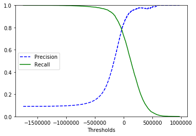
4. Precision / recall tradeoff
Precision은 다른 모든 양성 sample들(FN)을 무시하기 때문에 이들을 반영하는 recall과 반드시 함께 평가되어야 합니다. 안타깝게도 두 지표를 동시에 올릴 수는 없기 때문에 주어진 문제에 따라 가장 적절한 임곗값(threshold, decision function)을 정해야 합니다. 이를 precision / recall tradeoff 라고 부릅니다.
5. F$\bf{_1}$ score
F$\bf{_1}$ score 는 precision과 recall의 조화평균으로 precision과 recall이 비슷한 분류기에서 큰 값을 나타냅니다.
특히, 두 분류기를 비교할 때 precision과 recall을 하나의 지표로 만든 F$_1$ score를 편리하게 사용할 수 있습니다.
6. Micro / Macro average
Class가 3개 이상인 multi classification의 경우 confusion matrix는 다음과 같습니다.
| $P_1$ | $N_1$ | $P_2$ | $N_2$ | $P_3$ | $N_3$ | |
|---|---|---|---|---|---|---|
| $\hat P_1$ | $TP_1$ | $FP_1$ | ||||
| $\hat N_1$ | $FN_1$ | $TN_1$ | ||||
| $\hat P_2$ | $TP_2$ | $FP_2$ | ||||
| $\hat N_2$ | $FN_2$ | $TN_2$ | ||||
| $\hat P_3$ | $TP_3$ | $FP_3$ | ||||
| $\hat N_3$ | $FN_3$ | $TN_3$ |
Multi classification에서 class 전체의 평균을 구하는 방법으로 Micro average와 Macro average를 사용할 수 있습니다.
1) Micro average
\(\textbf{Precision}_{micro} = \frac{TP_1 + TP_2 + TP_3}{TP_1 + FP_1 + TP_2 + FP_2 + TP_3 + FP_3}\)
Micro average는 class를 나누지 않은 전체 성능의 양상을 알기에 적합합니다.
2) Macro average
\(\textbf{Precision}_{macro} = \frac{Precision_1 + Precision_2 + Precision_3}{3}\)
Class마다 데이터 수에 차이가 나는 경우 macro average를 사용하여 분포의 차이를 고려하여 성능을 평가할 수 있습니다.
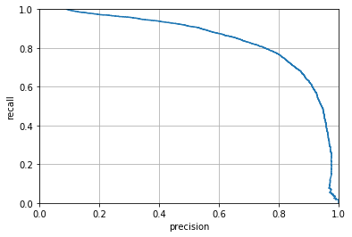
7. PR curve
Precision-recall graph를 말합니다.
일반적으로 precision이 급격하게 줄어드는 하강점 직전을 threshold로 정하는 것이 좋습니다. 어떤 precision이 주어지더라도 만족시키는 분류기를 만들 순 있지만, recall이 너무 낮다면 사용할 수 없기 때문에 생성된 분류기의 성능을 고려해야 합니다.
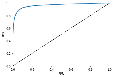
8. ROC curve (Receiver Operating Characteristic curve)
또다른 평가곡선으로 FPR-TPR graph를 ROC curve라 부릅니다.
FPR (False Positive Ratio, Type I error) 은 실제로 false$\color{red}{\textbf{(actual false)}}$인 sample들 중 true라고 예측$\color{green}{\textbf{(predictive true)}}$한 비율을 의미하며, TPR (True Positive Ratio, 1 - Type II error) 은 recall과 동일한 값을 나타냅니다. 여기서도 TPR(recall)이 높을수록 FPR이 증가하는 tradeoff가 발생합니다.
점선은 완전한 random 분류기를 의미하며 성능이 좋은 분류기는 이 점선으로부터 최대한 많이 떨어져 있는 (0, 1)에 근접한 모양이 됩니다. Curve 아래의 면적인 AUC(Area Under the Curve) 를 통해 분류기들을 비교할 수 있는데 완벽한 분류기는 AUC=1 이고, random 분류기의 AUC=0.5 가 됩니다.
일반적으로 true class가 적거나 FN보다 FP가 더 중요할 때 PR curve를 사용하고, 그 밖의 경우엔 ROC curve를 사용합니다.
3가지 그래프의 값들 모두 scikit-learn 의 함수들을 통해 얻을 수 있기 때문에 간단히 그릴 수 있습니다.
이 함수들에는 label과 분류기로부터 구할 수 있는 score (estimated probabilities or decision function)를 입력으로 받아들입니다,
대부분의 분류기들은 decision_function()을 가지고 있어 이 값을 score로 사용하지만 RandomForest와 같은 분류기들은 이 함수가 없는 대신 predict_proba()를 가지고 있어 이 값의 true estimated probabilities를 score로 사용합니다.
다음은 SGDClassifier와 RandomForestClassifier로부터 구한 곡선들을 그리는 코드입니다.2
1. Libraries and plotting function
1
2
3
4
5
import matplotlib.pyplot as plt
from sklearn.linear_model import SGDClassifier
from sklearn.ensemble import RandomForestClassifier
from sklearn.model_selection import cross_val_predict
from sklearn.metrics import precision_recall_curve, roc_curve, roc_auc_score
2. Score
1
2
3
4
5
6
sgd_clf = SGDClassifier(max_iter=5, random_state=42)
y_scores = cross_val_predict(sgd_clf, X_train, y_train, cv=3, method='decision_function')

forest_clf = RandomForestClassifier(random_state=42)
y_pred_proba = cross_val_predict(forest_clf, X_train, y_train, cv=3, method='predict_proba')
y_scores = y_pred_proba[:, 1]  # true class
3. PR curve 1
1
2
3
4
5
6
7
8
9
10
11
def plot_precision_recall_vs_threshold(precisions, recalls, thresholds):
    plt.plot(thresholds, precisions[:-1], 'b--', label='Precision')
    plt.plot(thresholds, recalls[:-1], 'g-', label='Recall')
    plt.xlabel('Thresholds')
    plt.legend(loc='center left')
    plt.ylim([0, 1])
    plt.grid()
    plt.show()

precisions, recalls, thresholds = precision_recall_curve(y_train, y_scores)
plot_precision_recall_vs_threshold(precisions, recalls, thresholds)
4. PR curve 2
1
2
3
4
5
6
7
8
9
def plot_precision_recall(precisions, recalls):
    plt.plot(precisions, recalls)
    plt.xlabel('Precision');  plt.ylabel('Recall')
    plt.axis([0, 1, 0, 1])
    plt.grid()
    plt.show()

precisions, recalls, thresholds = precision_recall_curve(y_train, y_scores)
plot_precision_recall(precisions, recalls)
5. ROC curve
1
2
3
4
5
6
7
8
9
10
def plot_roc_curve(fpr, tpr):
    plt.plot(fpr, tpr, linewidth=2)
    plt.plot([0, 1], [0, 1], 'k--')
    plt.axis([0, 1, 0, 1])
    plt.xlabel('FPR');  plt.ylabel('TPR')
    plt.show()

fpr, tpr, thresholds = roc_curve(y_train, y_scores)
plot_roc_curve(fpr, tpr)
print('AUC:', roc_auc_score(y_train, y_scores))