문제에 가장 적절한 모델을 찾은 후 해당 모델의 성능을 향상시키기 위한 방법을 찾기 위해 생겨난 에러의 종류를 분석할 수 있습니다. 이 과정을 에러 분석 (Error analysis) 라고 합니다.
0에서 9까지의 숫자 이미지를 분류하는 작업에서 linear SGDClassifier를 사용한 경우를 살펴봅시다.
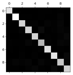
1. 먼저 confusion matrix를 구하고 matshow()를 사용하여 시각적으로 문제가 되는 지점을 분석합니다.
1
2
3
4
5
y_train_pred = cross_val_predict(sgd_clf, X_train_scaled, y_train, cv=3)
conf_mx = confusion_matrix(y_train, y_train_pred)

plt.matshow(conf_mx, cmap=plt.cm.gray)
plt.show()
2. 대응되는 클래스의 이미지 개수로 나누어 에러 비율을 비교합니다.
1
2
3
4
5
6
7
row_sums = conf_mx.sum(axis=1, keepdims=True)
norm_conf_mx = conf_mx / row_sums

# 그래프의 에러 부분에 초점을 맞추기 위해 잘한 부분은 0 처리
np.fill_diagonal(norm_conf_mx, 0)
plt.matshow(norm_conf_mx, cmap=plt.cm.gray)
plt.show()
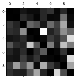
3. 에러 항들을 자세히 분석합니다.
1) 클래스 8과 9의 행과 열이 비교적 밝다
→ 많은 이미지가 8과 9로 잘못 분류되었다. 특히, 4와 7을 9로 잘못 분류한 sample이 많다
→ 그리고 8과 9 이미지를 다른 숫자로 분류한 경우가 많다. 특히, 9를 7로 잘못 분류한 sample이 많다
2) 클래스 0의 행과 열은 매우 어둡다
→ 대부분의 0 이미지들이 정확히 분류되었고, 다른 숫자 이미지들을 0 이라고 분류한 경우도 적다
3) 3-5, 7-9 pair가 상당히 밝다
→ 해당 pair의 이미지들을 더 모으거나 동심원의 수를 세는 알고리즘 등의 방법을 사용하여 개선할 필요가 있다
4. 여기서 3-5, 7-9 pair 이미지들을 confusion matrix 형식으로 출력해보았습니다.
1
2
3
4
5
6
7
8
9
10
11
12
13
14
15
16
17
18
19
20
21
22
23
24
25
26
27
28
29
30
def plot_digits(instances, images_per_row=10, **options):
    size = 28
    images_per_row = min(len(instances), images_per_row)
    images = [instance.reshape(size,size) for instance in instances]
    n_rows = (len(instances) - 1) // images_per_row + 1
    row_images = []
    n_empty = n_rows * images_per_row - len(instances)
    images.append(np.zeros((size, size * n_empty)))
    for row in range(n_rows):
        rimages = images[row * images_per_row : (row + 1) * images_per_row]
        row_images.append(np.concatenate(rimages, axis=1))
    image = np.concatenate(row_images, axis=0)
    plt.imshow(image, cmap = matplotlib.cm.binary, **options)
    plt.axis("off")

def plot_digit_confusion_mx(cl_a, cl_b):
    X_aa = X_train[(y_train == cl_a) & (y_train_pred == cl_a)]
    X_ab = X_train[(y_train == cl_a) & (y_train_pred == cl_b)]
    X_ba = X_train[(y_train == cl_b) & (y_train_pred == cl_a)]
    X_bb = X_train[(y_train == cl_b) & (y_train_pred == cl_b)]

    plt.figure(figsize=(8, 8))
    plt.subplot(221);  plot_digits(X_aa[:25], images_per_row=5)
    plt.subplot(222);  plot_digits(X_ab[:25], images_per_row=5)
    plt.subplot(223);  plot_digits(X_ba[:25], images_per_row=5)
    plt.subplot(224);  plot_digits(X_bb[:25], images_per_row=5)
    plt.show()

plot_digit_confusion_mx(3, 5)
plot_digit_confusion_mx(7, 9)
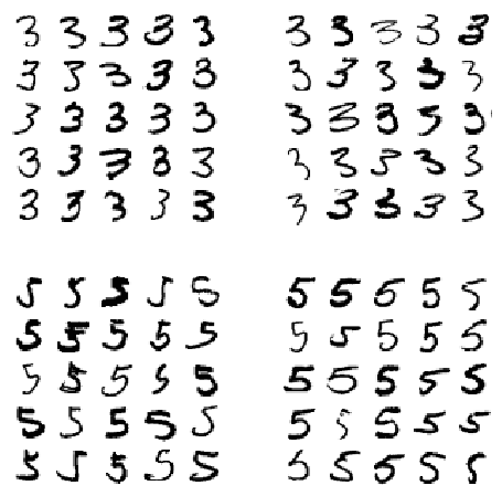
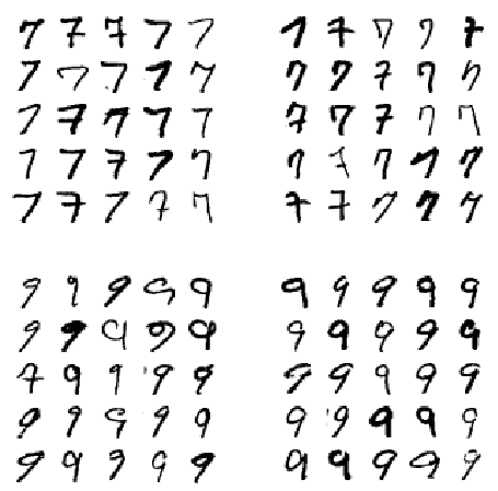
5. 결론
여기서 사용된 모델은 linear SGDClassifer 였습니다. 선형 분류기는 이미지에 대해 단순히 픽셀 강도의 가중치 합을 클래스의 점수로 사용하기 때문에 8과 9, 3과 5 그리고 7과 9 모두 몇 개의 픽셀만 다르기 때문에 모델이 쉽게 혼동할 수 있었던 것으로 생각해볼 수 있습니다.
PREVIOUSEtc