Decision Tree

Decision Tree
단계별로 각 feature의 적절한 값을 기준으로 sample들을 분할하여 tree 형태의 model을 학습시키는 방법이다. 매우 복잡한 데이터도 학습시킬 수 있는 강력한 알고리즘으로 분류와 회귀, 다중출력 작업도 가능한 다재다능한 알고리즘이다.

Remarks

본 포스팅은 Hands-On Machine Learning with Scikit-Learn & TensorFlow (Auérlien Géron, 박해선(역), 한빛미디어) 를 기반으로 작성되었습니다.

import os
import numpy as np
import matplotlib.pyplot as plt
%matplotlib inline

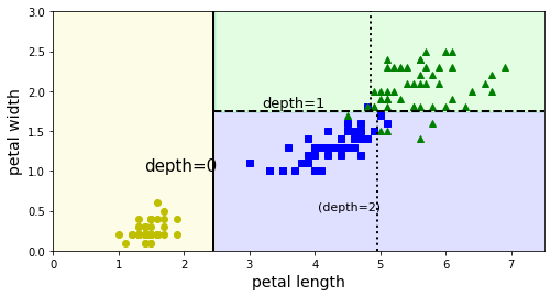
Classification Tree

from sklearn.datasets import load_iris
from sklearn.tree import DecisionTreeClassifier

iris = load_iris()
X, y = iris.data[:, 2:], iris.target

tree_clf = DecisionTreeClassifier(max_depth=2)
tree_clf.fit(X, y)

DecisionTreeClassifier(class_weight=None, criterion='gini', max_depth=2,
                       max_features=None, max_leaf_nodes=None,
                       min_impurity_decrease=0.0, min_impurity_split=None,
                       min_samples_leaf=1, min_samples_split=2,
                       min_weight_fraction_leaf=0.0, presort=False,
                       random_state=None, splitter='best')

from matplotlib.colors import ListedColormap

def plot_decision_boundary(clf, X, y, axes=[0, 7.5, 0, 3], iris=True, legend=False, plot_training=True):
    x1s = np.linspace(axes[0], axes[1], 100)
    x2s = np.linspace(axes[2], axes[3], 100)
    x1, x2 = np.meshgrid(x1s, x2s)
    X_new = np.c_[x1.ravel(), x2.ravel()]
    y_pred = clf.predict(X_new).reshape(x1.shape)
    custom_cmap = ListedColormap(['#fafab0','#9898ff','#a0faa0'])
    plt.contourf(x1, x2, y_pred, alpha=0.3, cmap=custom_cmap)
    if not iris:
        custom_cmap2 = ListedColormap(['#7d7d58','#4c4c7f','#507d50'])
        plt.contour(x1, x2, y_pred, cmap=custom_cmap2, alpha=0.8)
    if plot_training:
        plt.plot(X[:, 0][y==0], X[:, 1][y==0], "yo", label="Iris-Setosa")
        plt.plot(X[:, 0][y==1], X[:, 1][y==1], "bs", label="Iris-Versicolor")
        plt.plot(X[:, 0][y==2], X[:, 1][y==2], "g^", label="Iris-Virginica")
        plt.axis(axes)
    if iris:
        plt.xlabel("petal length", fontsize=14)
        plt.ylabel("petal width", fontsize=14)
    else:
        plt.xlabel(r"$x_1$", fontsize=18)
        plt.ylabel(r"$x_2$", fontsize=18, rotation=0)
    if legend:
        plt.legend(loc="lower right", fontsize=14)

plt.figure(figsize=(8, 4))
plot_decision_boundary(tree_clf, X, y)
plt.plot([2.45, 2.45], [0, 3], "k-", linewidth=2)
plt.plot([2.45, 7.5], [1.75, 1.75], "k--", linewidth=2)
plt.plot([4.95, 4.95], [0, 1.75], "k:", linewidth=2)
plt.plot([4.85, 4.85], [1.75, 3], "k:", linewidth=2)
plt.text(1.40, 1.0, "depth=0", fontsize=15)
plt.text(3.2, 1.80, "depth=1", fontsize=13)
plt.text(4.05, 0.5, "(depth=2)", fontsize=11)

plt.show()

png

from sklearn.tree import export_graphviz
import graphviz

def image_path(fig_id):
    if not os.path.isdir("DT"):
        os.mkdir("DT")
    return os.path.join("DT", fig_id)

file_path = image_path('iris_tree.dot')
export_graphviz(
    tree_clf,
    out_file=file_path,
    feature_names=['petal length', 'petal width'],
    class_names=iris.target_names,
    rounded=True,
    filled=True
)

with open(file_path) as f:
    dot_graph = f.read()
dot = graphviz.Source(dot_graph)
dot.format = 'png'
dot.render(filename='iris_tree', directory="DT", cleanup=True)
dot

svg

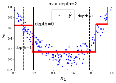
Regression Tree

from sklearn.tree import DecisionTreeRegressor

m = 200
X = np.random.rand(m, 1)
y = 4 * (X - 0.5)**2
y = y + np.random.randn(m, 1) / 10

tree_reg = DecisionTreeRegressor(max_depth=2)
tree_reg.fit(X, y)

DecisionTreeRegressor(criterion='mse', max_depth=2, max_features=None,
                      max_leaf_nodes=None, min_impurity_decrease=0.0,
                      min_impurity_split=None, min_samples_leaf=1,
                      min_samples_split=2, min_weight_fraction_leaf=0.0,
                      presort=False, random_state=None, splitter='best')

def plot_regression_predictions(tree_reg, X, y, axes=[0, 1, -0.2, 1], ylabel="$y$"):
    x1 = np.linspace(axes[0], axes[1], 500).reshape(-1, 1)
    y_pred = tree_reg.predict(x1)
    plt.axis(axes)
    plt.xlabel("$x_1$", fontsize=18)
    if ylabel:
        plt.ylabel(ylabel, fontsize=18, rotation=0)
    plt.plot(X, y, "b.")
    plt.plot(x1, y_pred, "r.-", linewidth=2, label=r"$\hat{y}$")

plot_regression_predictions(tree_reg, X, y)
for split, style in ((0.1973, "k-"), (0.0917, "k--"), (0.7718, "k--")):
    plt.plot([split, split], [-0.2, 1], style, linewidth=2)
plt.text(0.21, 0.65, "depth=0", fontsize=15)
plt.text(0.01, 0.2, "depth=1", fontsize=13)
plt.text(0.65, 0.8, "depth=1", fontsize=13)
plt.legend(loc="upper center", fontsize=18)
plt.title("max_depth=2", fontsize=14)
plt.show()

png

file_path = image_path("regression_tree.dot")
export_graphviz(
        tree_reg1,
        out_file=file_path,
        feature_names=["x1"],
        rounded=True,
        filled=True
    )

with open(file_path) as f:
    dot_graph = f.read()
dot = graphviz.Source(dot_graph)
dot.format = 'png'
dot.render(filename='regression_tree', directory='images/decision_trees', cleanup=True)
dot

svg

PREVIOUSEtc