Support Vector Machine

Support Vector Machine (SVM)은 선형, 비선형 분류, 회귀 이상치 탐색에도 사용할 수 있는 다목적 머신러닝 모델입니다.

Remarks

본 포스팅은 Hands-On Machine Learning with Scikit-Learn & TensorFlow (Auérlien Géron, 박해선(역), 한빛미디어) 를 기반으로 작성되었습니다.

I. Linear SVM Classification

Class 간의 가장 폭(margin)이 넓은 도로를 찾는 방법으로 생각할 수 있습니다. (large margin classification)
특히, 도로 경계에 위치하는 샘플들에 의해 결정 경계 (decision boundary)가 결정되기 때문에 이들을 support vector라고 부릅니다.

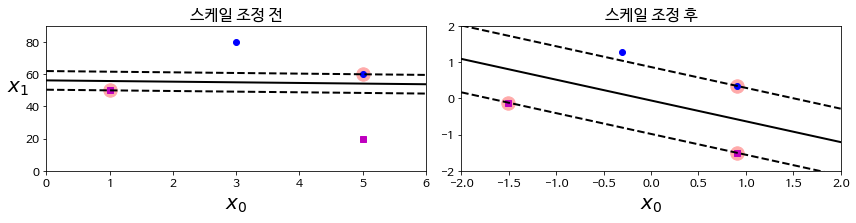
SVM은 scaling이 필요
각 feature의 scale의 차이가 크다면 margin이 작아질 수 있기 때문에 scaling이 필요하지만, 항상 그렇듯이 주어진 문제에 따라 적절히 적용하는 것이 바람직합니다.

png

1. Soft Margin Classification

모든 sample들이 도로 바깥쪽에 있도록 분류하는 hard margin classification이 거의 불가능하기 때문에 일반적으로 어느정도 도로 안쪽에도 샘플이 있는 것을 허용하는 soft margin classification을 사용합니다.

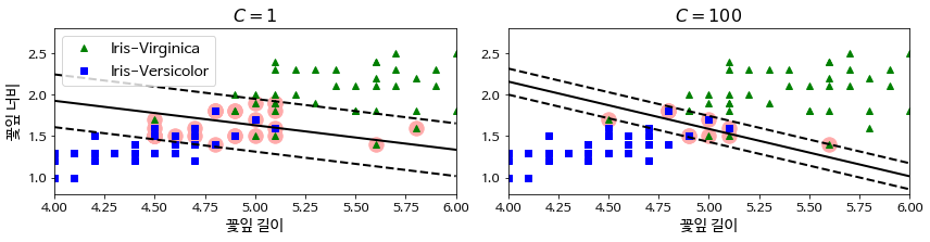
Hyperparameter: C
$ minimize_{w, b, \xi} \frac{1}{2} \mathbf{w}^T \mathbf{w} + $C$ \sum_i^m\xi$

Misclassification panelty. 작아질수록 도로의 폭이 넓어지지만, 도로 중간이나 심지어 반대쪽에 있는 샘플들의 개수가 많아집니다. 즉, margin violation(마진 오류)이 증가합니다.

Overfitting을 방지하기 위해 C를 감소 (C $ = \frac{1}{\lambda}$)
SVC(kernel='linear', C=1) 대신 LinearSVC(C=1, loss='hinge') 또는 SGDClassifier(loss='hinge', alpha=1/(m*C))를 사용
LinearSVC()는 bias를 포함하여 regularization를 수행하기 때문에 scaling이 꼭 필요
M > N 인 경우, LinearSVC(dual=False, C=1)
샘플의 개수가 feature의 개수보다 많은 경우, dual problem 대신 primal problem을 해결하는 것이 더 성능이 좋습니다. (loss='hinge'와 dual=False는 동시에 사용불가) 라고는 하지만.. dual=False로 하면 속도가 훨씬 느려지는 경우도 있으니 주의.

png

from sklearn import datasets
from sklearn.pipeline import Pipeline
from sklearn.preprocessing import StandardScaler
from sklearn.svm import LinearSVC
from sklearn.linear_model import LogisticRegression
from sklearn.model_selection import train_test_split
from sklearn.metrics import accuracy_score


iris = datasets.load_iris()
X, y = iris['data'][:, (2, 3)], (iris['target'] == 2).astype(np.float64)  # 꽃잎 길이, 너비 / Iris-Virginica
X_train, X_test, y_train, y_test = train_test_split(X, y, test_size=0.2, stratify=y)

svm_clf = Pipeline([
    ('scaler', StandardScaler()),
    ('linear_svc', LinearSVC(C=1, loss='hinge'))
    # SGDClassifier(loss='hinge', alpha=1/(m*C))
])
svm_clf.fit(X_train, y_train)
svm_pred = svm_clf.predict(X_test)
print(accuracy_score(svm_pred, y_test))

0.9333333333333333

def plot_dataset(X, y, axes):
    plt.plot(X[:, 0][y==0], X[:, 1][y==0], "bs")
    plt.plot(X[:, 0][y==1], X[:, 1][y==1], "g^")
    plt.axis(axes)
    plt.grid(True, which='both')
    plt.xlabel(r"$x_1$", fontsize=20)
    plt.ylabel(r"$x_2$", fontsize=20, rotation=0)

def plot_predictions(clf, axes):
    x0s = np.linspace(axes[0], axes[1], 100)
    x1s = np.linspace(axes[2], axes[3], 100)
    x0, x1 = np.meshgrid(x0s, x1s)
    X = np.c_[x0.ravel(), x1.ravel()]
    y_pred = clf.predict(X).reshape(x0.shape)
    y_decision = clf.decision_function(X).reshape(x0.shape)
    plt.contourf(x0, x1, y_pred, cmap=plt.cm.brg, alpha=0.2)
    plt.contourf(x0, x1, y_decision, cmap=plt.cm.brg, alpha=0.1)

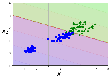
plot_predictions(svm_clf, [0, 8, -1, 4])
plot_dataset(X, y, [0, 8, -1, 4])
plt.show()

png

II. Nonlinear SVM Classification

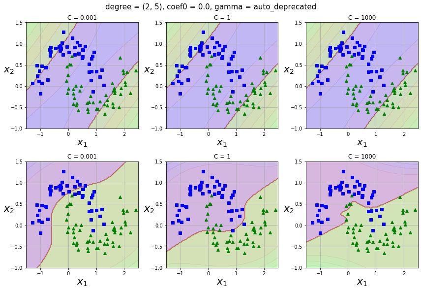
1. Polynomial Kernel

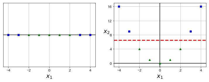
다항식 feature를 추가하는 것은 간단하고 모든 머신러닝 알고리즘에서 잘 작동하지만 feature의 개수가 많이 늘어나기 때문에 모델을 느리게 만듭니다. 그러나 SVM에서는 kernel trick을 통해 실제로는 feature를 추가하지 않으면서 다항식 feature를 많이 추가한 것과 동일한 결과를 얻을 수 있습니다.

png

Polynomial kernel
$K(\mathbf{x_1}, \mathbf{x_2}) = (\gamma \mathbf{x_1}^T\mathbf{x_2} + r)^d$

Hyperparameters: C (0.1 ~ 10), degree: $d$ (1 ~ 10), coef0: $r$ (0.1 ~ 10), gamma: $\gamma$ (1e-3 ~ 1e-1)
먼저 degree와 coef0를 적당한 값으로 고른다음, gamma(너무 큰 값 사용 X)와 C를 선택하는 것이 좋아보입니다.

SVC(C=1.0, kernel='rbf', degree=3, gamma='auto_deprecated', coef0=0.0,
    shrinking=True, probability=False, tol=0.001, cache_size=200, class_weight=None,
    verbose=False, max_iter=-1, decision_function_shape='ovr', random_state=None)

from sklearn.datasets import make_moons
from sklearn.pipeline import Pipeline
from sklearn.preprocessing import PolynomialFeatures
from sklearn.svm import SVC

X, y = make_moons(n_samples=100, noise=0.15, random_state=42)
polynomial_svm_clf = Pipeline([
    ('poly_features', PolynomialFeatures(degree=2)),
    ('scaler', StandardScaler()),
    ('svm_clf', LinearSVC(C=10, loss='hinge'))
])
poly_kernel_svm_clf = Pipeline([
    ('scaler', StandardScaler()),
    ('svm_clf', SVC(kernel='poly', degree=2, coef0=1, C=5))  # default: coef0=0
])

%%time
degrees = [2, 5]
Cs = [0.001, 1, 1000]
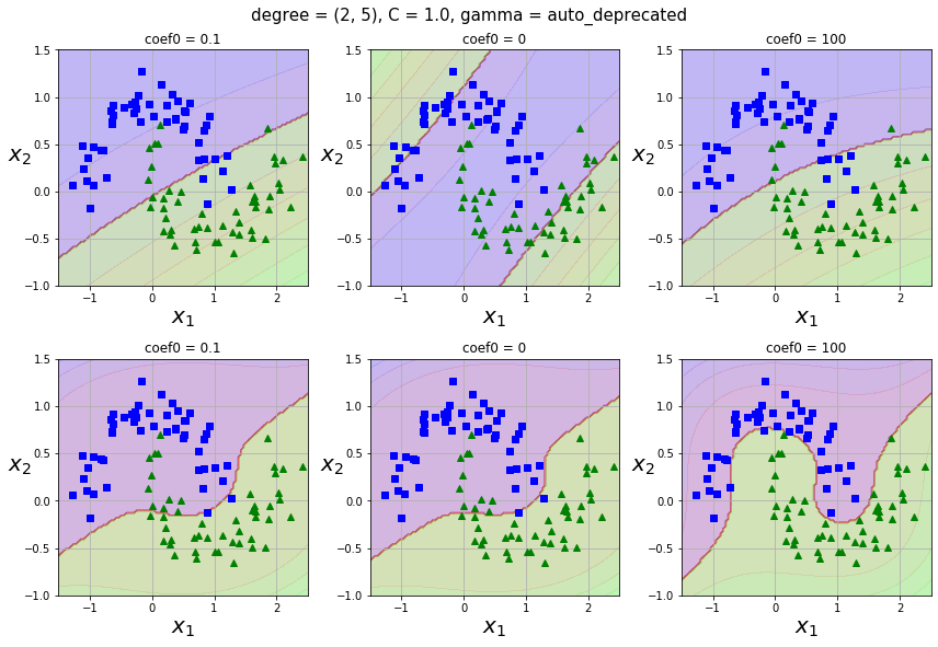
coef0s = [0.1, 0, 100]
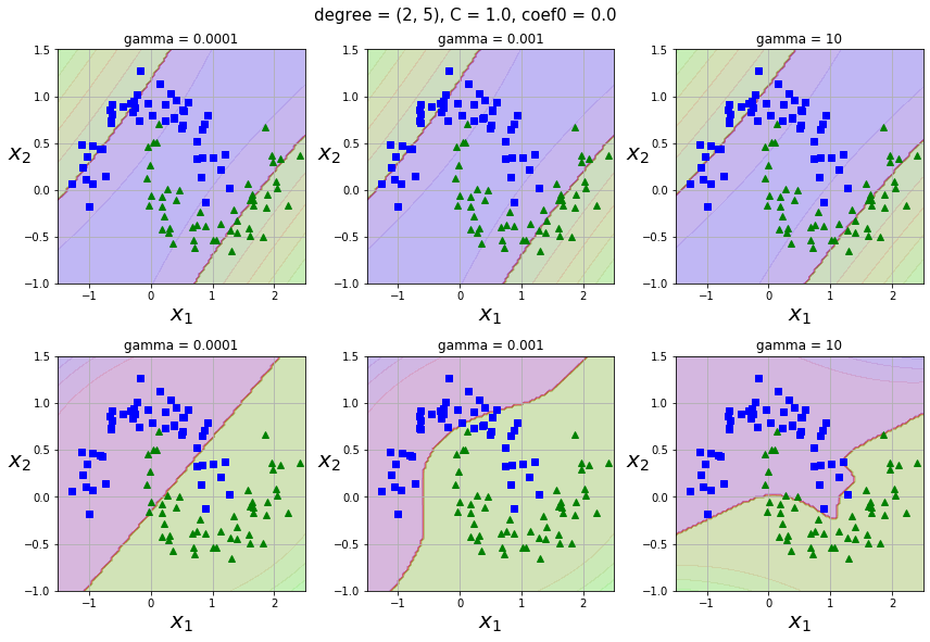
gammas = [0.0001, 0.001, 10]  # 큰 값이 들어오면 속도가 많이 떨어진다

svm_clfs = []
for degree in degrees:
    for C in Cs:
        svm_clf = Pipeline([
            ('scaler', StandardScaler()),
            ('svm_clf', SVC(kernel='poly', degree=degree, C=C))
        ])
        svm_clf.fit(X, y)
        svm_clfs.append(svm_clf)

for degree in degrees:
    for coef0 in coef0s:
        svm_clf = Pipeline([
            ('scaler', StandardScaler()),
            ('svm_clf', SVC(kernel='poly', degree=degree, coef0=coef0))
        ])
        svm_clf.fit(X, y)
        svm_clfs.append(svm_clf)

for degree in degrees:
    for gamma in gammas:
        svm_clf = Pipeline([
            ('scaler', StandardScaler()),
            ('svm_clf', SVC(kernel='poly', degree=degree, gamma=gamma))
        ])
        svm_clf.fit(X, y)
        svm_clfs.append(svm_clf)

# i = 0, 1, 2
for i, param in enumerate(('C', 'coef0', 'gamma')):
    _, a = plt.subplots(2, 3, figsize=(12, 8))
    s = 6 * i
    for j in range(6):
        plt.subplot(2, 3, 1 + j)
        clf = svm_clfs[s + j]

        params = {}
        clf_param = clf.get_params()
        for name in ('degree', 'C', 'coef0', 'gamma'):
            params[name] = clf_param['svm_clf__' + name]

        plt.title(f"{param} = {params[param]}")
        plot_dataset(X, y, [-1.5, 2.5, -1, 1.5])
        plot_predictions(clf, [-1.5, 2.5, -1, 1.5])
    if i == 0:
        plt.suptitle(f"degree = (2, 5), coef0 = {params['coef0']}, gamma = {params['gamma']}", fontsize=15, y=1.02)
    elif i == 1:
        plt.suptitle(f"degree = (2, 5), C = {params['C']}, gamma = {params['gamma']}", fontsize=15, y=1.02)
    elif i == 2:
        plt.suptitle(f"degree = (2, 5), C = {params['C']}, coef0 = {params['coef0']}", fontsize=15, y=1.02)
    plt.tight_layout()
plt.show()

png png png

CPU times: user 3.82 s, sys: 236 ms, total: 4.05 s
Wall time: 3.51 s

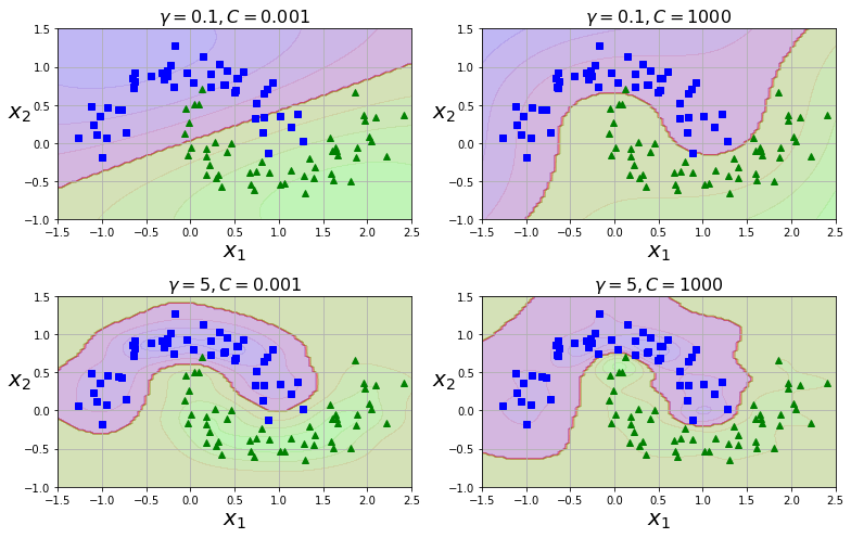
2. Gaussian RBF Kernel

Nonlinear feature을 다루는 또 다른 기법은 각 샘플이 특정 landmark와 얼마나 닮았는지 측정하는 유사도 함수(similarity function)로 계산한 특성을 추가하는 것입니다. 유사도 함수로는 주로 gaussian RBF(Radial Basis Function, 방사 기저 함수)를 사용합니다.

png

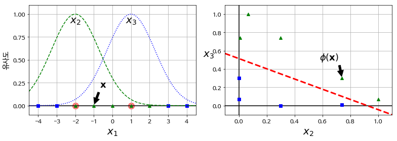
Gaussian RBF kernel
$\phi(\mathbf{x}, \mathbf{l}) = exp(-\gamma ||\mathbf{x} - \mathbf{l}||^2) $
Hyperparameters: C (0.1 ~ 10), gamma (1e-3 ~ 1e-1)
gamma를 증가시키면 종 모양 그래프가 좁아져서 각 샘플의 영향 범위가 작아집니다. 따라서 결정 경계가 조금 더 불규칙해지고 각 샘플을 따라 구불구불하게 휘어집니다. Overfitting을 방지하기 위해 gamma를 작게 하는 것 (C도 작게)이 도움이 됩니다.
Computational complexity
LinearSVC()의 경우 primal problem을 풀어 $O(mn)$ 으로 낮은 편이지만, SVC()의 경우 dual problem을 풀기 때문에 $O(m^2n) \sim O(m^3n)$ 사이로 수십만 개의 샘플을 학습시키는 데에는 적절하지 않습니다.

gamma1, gamma2 = 0.1, 5
C1, C2 = 0.001, 1000
hyperparams = (gamma1, C1), (gamma1, C2), (gamma2, C1), (gamma2, C2)

svm_clfs = []
for gamma, C in hyperparams:
    rbf_kernel_svm_clf = Pipeline([
            ("scaler", StandardScaler()),
            ("svm_clf", SVC(kernel="rbf", gamma=gamma, C=C))
        ])
    rbf_kernel_svm_clf.fit(X, y)
    svm_clfs.append(rbf_kernel_svm_clf)

plt.figure(figsize=(11, 7))

for i, svm_clf in enumerate(svm_clfs):
    plt.subplot(221 + i)
    plot_predictions(svm_clf, [-1.5, 2.5, -1, 1.5])
    plot_dataset(X, y, [-1.5, 2.5, -1, 1.5])
    gamma, C = hyperparams[i]
    plt.title(r"$\gamma = {}, C = {}$".format(gamma, C), fontsize=16)

plt.tight_layout()
plt.show()

png

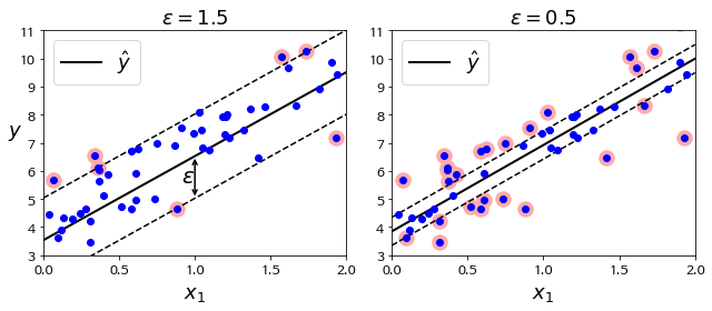
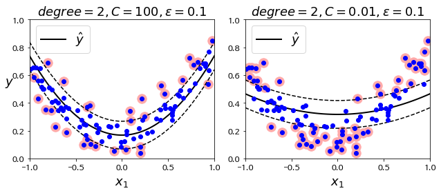
III. SVM Regression

Classification과 목표를 반대로 잡으면 regression에 SVM을 사용할 수 있습니다.
제한된 margin violation 안에서 도로 안에 가능한 많은 샘플이 들어가도록 학습합니다. 도로의 폭은 hyperparameter epsilon으로 조절합니다.

png png

IV. MNIST Classification Example

1. Load libraries

from sklearn.datasets import fetch_openml
from sklearn.model_selection import train_test_split
from sklearn.pipeline import Pipeline
from sklearn.preprocessing import StandardScaler
from sklearn.metrics import accuracy_score
from sklearn.svm import LinearSVC, SVC
from sklearn.model_selection import RandomizedSearchCV
from scipy.stats import reciprocal, uniform

2. Load dataset and split

mnist = fetch_openml('mnist_784', version=1)
X, y = mnist['data'], mnist['target']
X_train_val, X_test, y_train_val, y_test = train_test_split(X, y, test_size=1/7, stratify=y)
X_train, X_val, y_train, y_val = train_test_split(X_train_val, y_train_val, test_size=1/6, stratify=y_train_val)
_, X_train_10000, _, y_train_10000 = train_test_split(X_train, y_train, test_size=10000, stratify=y_train)
_, X_train_1000, _, y_train_1000 = train_test_split(X_train, y_train, test_size=1000, stratify=y_train)

print(X_train.shape, X_test.shape, X_train_val.shape, X_val.shape)
print(X_train_10000.shape, X_train_1000.shape)

(50000, 784) (10000, 784) (60000, 784) (10000, 784)
(10000, 784), (1000, 784)

3. Define foundation models

linear_clf = Pipeline([
    ('std_scaler', StandardScaler()),
    ('svm_clf', LinearSVC(random_state=42))  # C
])

poly_clf = Pipeline([
    ('std_scaler', StandardScaler()),
    ('svm_clf', SVC(kernel='poly', coef0=10, random_state=42))  # C, gamma, coef0, degree
])

rbf_clf = Pipeline([
    ('std_scaler', StandardScaler()),
    ('svm_clf', SVC(kernel='rbf', random_state=42))  # C, gamma
])

4. Check accuracy with small dataset

models = [linear_clf, poly_clf, rbf_clf]
names = ['linear svm', 'polynomial svm', 'rbf svm']
for model, name in zip(models, names):
    print(f"<{name}>")
    %time model.fit(X_train_10000, y_train_10000)
    y_train_10000_pred, y_val_pred = model.predict(X_train_10000), model.predict(X_val)
    acc_train, acc_val = accuracy_score(y_train_10000, y_train_10000_pred), accuracy_score(y_val, y_val_pred)
    print(f"{name} | acc_train: {acc_train} \t val_train: {acc_val} \n")

<linear svm>
CPU times: user 19.3 s, sys: 4 ms, total: 19.3 s
Wall time: 19.3 s
linear svm | acc_train: 0.9795 	 val_train: 0.8847

※ 5,000개 샘플을 학습시킨 경우,
CPU times: user 7.44 s, sys: 1 µs, total: 7.44 s
Wall time: 7.43 s
linear svm | acc_train: 0.9986 	 val_train: 0.8359


<polynomial svm>
CPU times: user 4.56 s, sys: 244 ms, total: 4.8 s
Wall time: 4.4 s
polynomial svm | acc_train: 1.0 	 val_train: 0.9245

※ 5,000개 샘플을 학습시킨 경우,
CPU times: user 1min 14s, sys: 188 ms, total: 1min 14s
Wall time: 1min 14s
polynomial svm | acc_train: 0.9215 	 val_train: 0.8871


<rbf svm>
CPU times: user 29.3 s, sys: 4.01 ms, total: 29.3 s
Wall time: 29.3 s
rbf svm | acc_train: 0.9817 	 val_train: 0.9479

※ 5,000개 샘플을 학습시킨 경우,
CPU times: user 9.57 s, sys: 0 ns, total: 9.57 s
Wall time: 9.57 s
rbf svm | acc_train: 0.9778 	 val_train: 0.9294

rbf_clf를 개선하기로 결정

5. Hyperparameter tuning

param_distributions = {"svm_clf__gamma": reciprocal(1e-3, 1e-1), "svm_clf__C": uniform(1, 10)}
rnd_search_cv = RandomizedSearchCV(rbf_clf, param_distributions, cv=3, n_iter=10, verbose=2, n_jobs=-1)
rnd_search_cv.fit(X_train_1000, y_train_1000)

Fitting 3 folds for each of 10 candidates, totalling 30 fits
[Parallel(n_jobs=-1)]: Using backend LokyBackend with 6 concurrent workers.
[Parallel(n_jobs=-1)]: Done  30 out of  30 | elapsed:    5.3s finished

best_model = rnd_search_cv.best_estimator_
print(rnd_search_cv.best_score_)

0.822

%time best_model.fit(X_train_val, y_train_val)
y_test_pred = best_model.predict(X_test)
print(accuracy_score(y_test, y_test_pred))

0.9709

PREVIOUSEtc