import time
import numpy as np
import matplotlib
import matplotlib.pyplot as plt

from sklearn import svm
from sklearn.datasets import make_moons, make_blobs
from sklearn.covariance import EllipticEnvelope
from sklearn.ensemble import IsolationForest
from sklearn.neighbors import LocalOutlierFactor

matplotlib.rcParams['contour.negative_linestyle'] = 'solid'

print(__doc__)

# Example settings

n_samples = 300
outliers_fraction = 0.15
n_outliers = int(outliers_fraction * n_samples)
n_inliers = n_samples - n_outliers

# Define outlier / anomaly detection methods to be compared

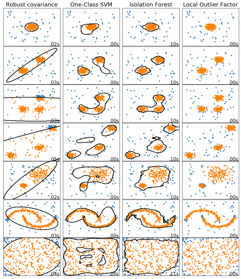
anomaly_algorithms = [
    ("Robust covariance", EllipticEnvelope(contamination=outliers_fraction)),
    ("One-Class SVM", svm.OneClassSVM(nu=outliers_fraction,
                                      kernel='rbf',
                                      gamma=0.1)),
    ("Isolation Forest", IsolationForest(behaviour='new',
                                         contamination=outliers_fraction,
                                         random_state=42)),
    ("Local Outlier Factor", LocalOutlierFactor(n_neighbors=35,
                                                contamination=outliers_fraction))
]

# Define datasets

blobs_params = dict(random_state=0, n_samples=n_inliers, n_features=2)
datasets = [
    make_blobs(centers=[[0, 0], [0, 0]], cluster_std=0.5, **blobs_params)[0],
    make_blobs(centers=[[2, 2], [-2, -2]], cluster_std=[0.5, 0.5], **blobs_params)[0],
    make_blobs(centers=[[2, 2], [-2, -2], [2, -2]], cluster_std=[0.5, 0.5, 0.5], **blobs_params)[0],
    make_blobs(centers=[[5, 5], [-5, -5], [2, -2]], cluster_std=[0.5, 0.5, 0.5], **blobs_params)[0],
    make_blobs(centers=[[2, 2], [-2, -2]], cluster_std=[1.5, 0.3], **blobs_params)[0],
    4. * (make_moons(n_samples=n_samples, noise=0.05, random_state=0)[0] - np.array([0.5, 0.25])),
    14. * (np.random.RandomState(42).rand(n_samples, 2) - 0.5)
]

# Compare given classifiers under given settings

xx, yy = np.meshgrid(np.linspace(-7, 7, 150),
                     np.linspace(-7, 7, 150))

plt.figure(figsize=(len(anomaly_algorithms) * 2 + 3, 12.5))
plt.subplots_adjust(left=0.02, right=0.98, bottom=0.001, top=0.96, wspace=0.05, hspace=0.01)

plot_num = 1
rng = np.random.RandomState(42)

for i_dataset, X, in enumerate(datasets):
    # Add outliers
    X = np.concatenate([X, rng.uniform(low=-6, high=6, size=(n_outliers, 2))], axis=0)

    for name, algorithm in anomaly_algorithms:
        t0 = time.time()
        algorithm.fit(X)
        t1 = time.time()
        plt.subplot(len(datasets), len(anomaly_algorithms), plot_num)

        if i_dataset == 0:
            plt.title(name, size=18)

        # Fit the data and tag outliers
        if name == "Local Outlier Factor":
            y_pred = algorithm.fit_predict(X)
        else:
            y_pred = algorithm.fit(X).predict(X)

        # Plot the levels lines and the points
        if name != "Local Outlier Factor":
            Z = algorithm.predict(np.c_[xx.ravel(), yy.ravel()])
            Z = Z.reshape(xx.shape)
            plt.contour(xx, yy, Z, levels=[0], linewidths=2, colors='black')

        colors = np.array(['#377eb8', '#ff7f00'])
        plt.scatter(X[:, 0], X[:, 1], s=10, color=colors[(y_pred + 1) // 2])

        plt.xlim(-7, 7);  plt.ylim(-7, 7)
        plt.xticks(());  plt.yticks(())
        plt.text(0.99, 0.01, ('%.2fs' % (t1 - t0)).lstrip('0'),
                 transform=plt.gca().transAxes, size=15,
                 horizontalalignment='right')
        plot_num += 1

plt.show()