Remarks
본 글은 한양대학교 이기천 교수님의 시계열분석 강의 3강을 정리한 글입니다.
이전 강의까지 trend를 찾아내는 몇 가지 방법들을 배웠다.
찾아낸 trend를 제거하면 residual이 남게 되는데, 이번 강의부터는 residual을 modeling하는 방법에 대해 배운다.
1. Autoregressive model
1) AR(1)
\(\begin{equation} \begin{aligned} x_t &= \phi x_{t-1} + a_t + \mu \\ &= \phi(\phi x_{t-2} + a_{t-1} + \mu) + a_t + \mu \\ &= \ ... \\ &= a_t + \phi a_{t-1} + \phi^2 a_{t-2} + \cdots \\ &\ \quad \mu + \phi \mu + \phi^2 \mu + \cdots \\ &= \phi^m x_{t-m} + \phi^{m-1} a_{t-(m-1)} + \cdots + a_t + (\phi^{m-1} + \cdots + 1) \mu \\ &\approx a_t + \cdots + \phi^{m-1} a_{t-(m-1)} + (1 + \cdots + \phi^{m-1}) \mu \quad \text{ if } \mid \phi \mid < 1 \text{ and } m \text{ is sufficiently large} \\ &\approx a_t + \cdots + \phi^{m-1} a_{t-(m-1)} + \frac{\mu}{1 - \phi} \end{aligned} \end{equation}\)
- Expectation
\(\begin{equation} \begin{aligned} E(x_t) &= E(\phi x_{t-1} + a_t + \mu) \\ &= \phi E(x_{t-1}) + \mu \quad \text{ if } \ E(x_t) = E(x_{t-1}) \\ E(x_t) &= \frac{\mu}{1-\phi} \end{aligned} \end{equation}\)
즉, $\mid \phi \mid < 1$ 조건이 주어졌을 때, 그리고 $E(x_t)$와 $E(x_t) = E(x_{t-1}$ 조건이 주어졌을 때의 $E(x_t)$가 $\frac{\mu}{1 - \phi}$로 동일하다.
- Variance
\(\begin{equation} \begin{aligned} Var(x_t) &= Var(a_t + \cdots + \phi^{m-1} a_{t-(m-1)} + \frac{\mu}{1 - \phi}) \\ &= Var(a_t) + \cdots + \phi^{2(m-1)} Var(a_{t-(m-1)}) \\ &= \sigma^2 + \cdots + \phi^{2(m-1)}\sigma^2 \\ &= \frac{\sigma^2}{1 - \phi^2} \\ \end{aligned} \end{equation}\)
Expectation과 마찬가지로, $\mid \phi \mid < 1$ 조건에서 $Var(x_t) = Var(x_{t-1})$ 조건이 주어진 경우와 동일한 결과를 보인다.
- Covariance
$Cov(x_t, a_{t+1}) = 0$
왜냐하면 $x_t$는 $a_t, a_{t-1}, \cdots$ 들로 구성되지만, $a_{t-h}$는 $a_{t+1}$과 독립이기 때문에 covariance가 0이다.
2) Causality
$x_t = f(a_t, a_{t-1}, \cdots)$ 인 system을 causal system이라고 한다.
즉, 현재의 observation이 현재의 noise와 이전의 noise들에 의해서 표현되는 system을 causal system이라고 부른다.
Observation $x_t$를 random variable $a_t$들로 나타낸다면, 통계학적으로 여러가지를 말할 수 있게된다. (confidence interval 등)
-
Causal ARMA model
$x_t = \theta_0 a_t - \theta_1 a_{t-1} - \cdots$ ($\theta_0 = 1$)
$\sum_{j=0}^\infty \mid \theta_j \mid < \infty$ (bounded)
AR(1)이 causal ARMA model이 되기 위해선, $\mid \phi \mid < 1$ 조건이 필요하다. (stationary 조건과 동일)
ex) $x_t = 2x_{t-1} - a_t$ 는 causal system이 아니다.
\(\begin{equation} \begin{aligned} x_t &= 2x_{t-1} - a_t \\ x_{t-1} &= \frac{1}{2}x_t + \frac{a_t}{2} \\ &= \frac{a_t}{2} + \frac{a_{t+1}}{2^2} + \frac{x_{t+1}}{2^2} \\ &= \frac{a_t}{2} + \frac{a_{t+1}}{2^2} + \frac{a_{t+2}}{2^3} + \cdots \end{aligned} \end{equation}\)
혹은,
\(\begin{equation} \begin{aligned} x_t &= 2x_{t-1} - a_t \\ &= 2^m x_{t-m} + 2^{m-1}a_{t-(m-1)} + \cdots + 2 a_{t-1} + a_t \end{aligned} \end{equation}\)
Stationary하지만, causal system은 아니다. -
Stationary and Causal system
우리가 분석할 대상은 stationary 하면서도 causal한 system이다.
이를 위해 causal model을 가정한다. ($x_t$ and $a_{t+1}$ are not correlated)
3) Beyond AR(1)
- AR(1)
\(\begin{equation} \begin{aligned} x_t &= \phi x_{t-1} + a_t + \mu \quad \cdots \text{ constant } \mu \text{ can be removed by centering} \\ &= \phi Bx_t + a_t + \mu \\ x_t - \phi Bx_t &= a_t + \mu \\ (1 - \phi B)x_t &= a_t + \mu \\ x_t &= \frac{1}{1 - \phi B} (a_t + \mu ) \quad \cdots \text{ causal expression} \\ &= (1 + \phi B + \phi^2 B^2 + \cdots) (a_t + \mu ) \quad \text{ if } \ \mid \phi \mid < 1 \\ &= a_t + \phi a_{t-1} + \phi^2 a_{t-2} + \cdots + \\ &\ \quad \ \mu + \phi \mu + \phi^2 \mu + \cdots \end{aligned} \end{equation}\)
- AR(2)
\(\begin{equation} \begin{aligned} x_t &= \phi_1 x_{t-1} + \phi_2 x_{t-2} + a_t + \mu \quad \cdots \text{ constant } \mu \text{ can be removed by centering} \\ &= \phi_1 Bx_t + \phi_2 B^2x_t + a_t + \mu \\ x_t - \phi_1 Bx_t - \phi_2 B^2x_t &= a_t + \mu \\ (1 - \phi_1 B - \phi_2 B^2)x_t &= a_t + \mu \\ (1 - \alpha_1B)(1 - \alpha_2B)x_t &= a_t + \mu \\ x_t &= \frac{1}{(1 - \alpha_1B)(1 - \alpha_2B)} (a_t + \mu ) \quad \cdots \text{ causal expression} \\ &= \frac{1}{1 - \alpha_1B} \frac{1}{1 - \alpha_2B}(a_t +\mu) \\ &= (1 + \alpha_1 B + \alpha_1^2 B^2 + \cdots) (1 + \alpha_2 B + \alpha_2^2 B^2 + \cdots) (a_t + \mu ) \quad \text{ if } \ \mid \alpha_1 \mid < 1 \text{ and } \mid \alpha_2 \mid < 1 \\ &= (1 + (\alpha_1 + \alpha_2)B + (\alpha_1^2 + \alpha_1 \alpha_2 + \alpha_2^2)B^2 + \cdots)(a_t + \mu) \\ &= a_t + \beta_1 a_{t-1} + \beta_2 a_{t-2} + \cdots + \\ &\ \quad \ \mu + \gamma_1 \mu + \gamma_2 \mu + \cdots \end{aligned} \end{equation}\)
한편, 등비급수로 표현(invertible)되기 위한 조건은 다음과 같이 $\phi$에 대한 식으로 변경될 수 있다.
\(\begin{equation}
\begin{aligned}
&\ \mid \alpha_1 \mid < 1 \text{ and } \mid \alpha_2 \mid < 1 \\
&\Leftrightarrow \ \phi_1 + \phi_2 < 1 \text{ and } \phi_2 - \phi_1 < 1 \text{ and } \mid \phi_2 \mid < 1
\end{aligned}
\end{equation}\)
- AR(3)
\(\begin{equation}
\begin{aligned}
x_t &= \phi_1 x_{t-1} + \phi_2 x_{t-2} + \phi_3 x_{t-3} + a_t + \mu \quad \cdots \text{ constant } \mu \text{ can be removed by centering} \\
&= \phi_1 Bx_t + \phi_2 B^2x_t + \phi_3 B^3x_t + a_t + \mu \\
x_t - \phi_1 Bx_t - \phi_2 B^2x_t - \phi_3 B^3x_t &= a_t + \mu \\
(1 - \phi_1 B - \phi_2 B^2 - \phi_3 B^3)x_t &= a_t + \mu \\
(1 - \alpha_1B)(1 - \alpha_2B)(1 - \alpha_3B)x_t &= a_t + \mu \\
\end{aligned}
\end{equation}\)
지금까지 한 것은 AR(1)부터 expectation, variance를 구하고 stationary, invertible 하게 표현할 수 있는 조건을 찾아내었다.
그리고 recursive하게 적어 causal하게 표현될 수 있는 조건을 찾았다. (모두 동일)
AR(2), AR(3) 역시 AR(1)과 마찬가지로 유사한 식으로 표현된다는 것을 확인하였다.
ex) AR(2): $x_t = x_{t-1} - 0.89 x_{t-2} + a_t$
- $(1 - B + 0.89 B^2)x_t = a_t$
- $(1 - (0.5 + 0.8i))(1 + (0.5 - 0.8i))x_t = a_t$
- $x_t = a_t + \psi_1 a_{t-1} + \psi_2 a_{t-2} + \cdots$ ($\psi_1 = \alpha_1 + \alpha_2 = 1$, $\psi_2 = \alpha_1^2 + \alpha_2^2 + \alpha_1 \alpha_2 = 0.11$)
⇒ $x_t$ is stationary and causal
이와 같이 AR model에서 coefficient가 주어진 경우, causal expression에서 coefficient를 구할 수 있고 $x_t$의 stationarity와 causality도 알 수 있다.
4) Appropriate order of AR
주어진 time series에 적절한 model을 정하기 위해, autocovariance / autocorrelation function $\gamma_x(h)$ 혹은 $\rho_x(h)$를 이용한다.
2. Yule-Walker equation
For example, how do we relate $\gamma_x(h)$ or $\rho_x(h)$ to AR(2)?
$\phi$를 예측하기 위해 $\gamma_x(h)$, $\rho_x(h)$이 model과 어떻게 연관되어 있는지 알려주는 식이 Yule-Walker equation이다.
- AR(2)
\(\begin{equation} \begin{aligned} x_t &= \phi_1 x_{t-1} + \phi_2 x_{t-2} + a_t + \mu \\ x_t x_{t-h} &= \phi_1 x_{t-1} x_{t-h} + \phi_2 x_{t-2} x_{t-h} + a_t x_{t-h} + \mu x_{t-h} \quad \cdots \text{ multiply } x_{t-h} \\ E(x_t x_{t-h}) &= E(\phi_1 x_{t-1} x_{t-h} + \phi_2 x_{t-2} x_{t-h} + a_t x_{t-h} + \mu x_{t-h}) \\ &= \phi_1 E(x_{t-1} x_{t-h}) + \phi_2 E(x_{t-2} x_{t-h}) + E(a_t x_{t-h}) + \mu E(x_{t-h}) \\ \\ \text{if $h = 0$,} \\ E(x_t x_{t-0}) &= E(x_t^2) = Var(x_t) = \gamma_x(0) \quad \cdots \text{ assume } E(x_t) = 0 \\ &= \phi_1 E(x_{t-1} x_{t}) + \phi_2 E(x_{t-2} x_{t}) + E(a_t x_t) + \mu E(x_t) \\ &= \phi_1 \gamma_x(1) + \phi_2 \gamma_x(2) + \sigma^2 \quad \cdots \ E(a_t x_t) = Cov(a_t, x_t) = Cov(a_t, a_t + \psi_1 a_{t-1} + \cdots) = Var(a_t) \\ \\ \text{if $h = 1$,} \\ E(x_t x_{t-1}) &= Cov(x_t, x_{t-1}) = \gamma_x(1) \quad \cdots \text{ assume } E(x_t) = 0 \\ &= \phi_1 E(x_{t-1} x_{t-1}) + \phi_2 E(x_{t-2} x_{t-1}) + E(a_t x_{t-1}) + \mu E(x_{t-1}) \\ &= \phi_1 \gamma_x(0) + \phi_2 \gamma_x(1) \quad \cdots \ E(a_t x_{t-1}) = Cov(a_t, x_{t-1}) = Cov(a_t, a_{t-1} + \psi_1 a_{t-2} + \cdots) = 0 \\ \\ \text{if $h = 2$,} \\ E(x_t x_{t-2}) &= Cov(x_t, x_{t-2}) = \gamma_x(2) \quad \cdots \text{ assume } E(x_t) = 0 \\ &= \phi_1 E(x_{t-1} x_{t-2}) + \phi_2 E(x_{t-2} x_{t-2}) + E(a_t x_{t-2}) + \mu E(x_{t-2}) \\ &= \phi_1 \gamma_x(1) + \phi_2 \gamma_x(0) \quad \cdots \ E(a_t x_{t-2}) = Cov(a_t, x_{t-2}) = Cov(a_t, a_{t-2}+ \psi_1 a_{t-3} + \cdots) = 0 \\ \\ \text{for $h > 2$,} \\ E(x_t x_{t-h}) &= \gamma_x(h) \\ \gamma_x(h) &= \phi_1 \gamma_x(h-1) + \phi_2 \gamma_x(h-2) \end{aligned} \end{equation}\)
1) Yule-Walker equation
\(\gamma_x(h)-\phi_1 \gamma_x(h-1) - \phi_2 \gamma_x(h-2) = \begin{cases} \sigma^2 & \quad \text{if } h = 0 \\ 0 & \quad \text{if } h \geq 1 \\ \end{cases}\)
- Autocorrelation
$\rho_x(h) = \frac{\gamma_x(h)}{\gamma_x(0)}, \rho_x(0) = 1$
\(\begin{aligned} \rho_x(h) = 1 \quad &\text{if } h = 0 \\ \rho_x(h)-\phi_1 \rho_x(h-1) - \phi_2 \rho_x(h-2) = 0 \quad &\text{if } h \geq 1 \end{aligned}\)
2) Find $\phi$ from $\rho(h)$
\[\begin{aligned} \text{if } h = 1, \quad \quad \quad \quad \quad \quad \quad \quad \quad \\ \rho_x(1) - \phi_1 \rho_x(0) - \phi_2 \rho_x(1) &= 0 \\ \rho_x(1) - \phi_1 - \phi_2 \rho_x(1) &= 0 \\ \\ \text{if } h = 2, \quad \quad \quad \quad \quad \quad \quad \quad \quad \\ \rho_x(2) - \phi_1 \rho_x(1) - \phi_2 \rho_x(0) &= 0 \\ \rho_x(2) - \phi_1 \rho_x(1) - \phi_2 &= 0 \\ \end{aligned}\]주어진 time series로부터 $\rho(h)$를 구할 수 있고, 이로부터 얼마든지 $\phi$를 계산해낼 수 있다.
\(\begin{cases}
\rho_x(1) - \phi_1 - \phi_2 \rho_x(1) = 0 \\
\rho_x(2) - \phi_1 \rho_x(1) - \phi_2 = 0 \\
\end{cases}\)
ex)
Observations: $x_1, \cdots x_{144}$ ($n=144$)
Assume AR(2) model: $x_t = \phi_1 x_{t-1} + \phi_2 x_{t-2} + a_t$ (나중에 어떤 model이 좋은지 설명)
Estimate $\phi_1, \phi_2$
- Compute $\hat \gamma(1), \hat \gamma(2)$
\(\begin{aligned} \gamma(h) &= Cov(x_t, x_{t-h}) \\ &= E[(x_t - \mu) (x_{t-h} - \mu)] \quad \cdots \ \mu \equiv E(x_t) \\ \hat \gamma(h) &= \frac{1}{n-h} \sum_{t = h+1}^n (x_t - \bar x)(x_{t-h} - \bar x) \quad \cdots \ \bar x \equiv \frac{1}{n} \sum_t x_t \end{aligned}\) - Compute $\hat \rho(1), \hat \rho(2)$
$\hat \rho(h) = \frac{\hat \gamma(h)}{\gamma(0)}$
- Use Y-K equations for AR(2)
\(\begin{cases} \hat \rho_x(1) - \phi_1 - \phi_2 \hat \rho_x(1) = 0 \\ \hat \rho_x(2) - \phi_1 \hat \rho_x(1) - \phi_2 = 0 \\ \end{cases}\)
⇒ $\hat \phi_1 \hat \phi_2$
- What about variability of WN $\sigma^2$?
Use Y-K equation with $\gamma(0)$
$\hat \gamma_x(0)- \hat \phi_1 \hat \gamma_x(1) - \hat \phi_2 \hat \gamma_x(2) = \hat \sigma^2$
⇒ $\hat \sigma^2$
3) Deep into the $\rho_x(h)$
Data로부터 계산할 수 있는 $\rho_x(h)$와 model간의 관계를 자세히 알아보자.
- AR(1)
AR(1): $x_t = \phi_1 x_{t-1} + a_t \quad \cdots \quad$ stationary if $\mid \phi_1 \mid < 1$
양변에 $x_{t-h}$를 곱해주고 expectation을 취하는 Y-K equation을 만들어주면,
Y-W eq: $\rho(h) = \phi_1 \rho(h-1), \ h \geq 1$
즉, $\rho(h) = \phi_1^h$ 이다.
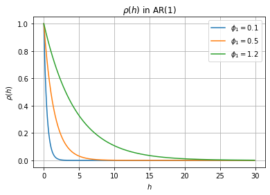
만약 data로부터 구한 $\rho(h)$가 $h$에 exponential한 관계를 보인다면, 이것은 AR(1) model을 사용하는 것이 좋다는 clue가 된다.
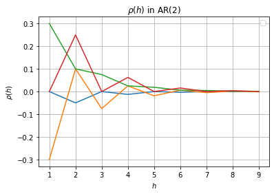
- AR(2)
Y-W eq: $\rho(h) = \phi_1 \rho(h-1) + \phi_2 \rho(h-2)$
$\rho(h) = a_1 y_1^h + a_2 y_2^h \quad \cdots \quad y_1, y_2 \text{: solution of } y^2 - \phi_1 y - \phi_2 = 0, \ a \text{: solved by } \rho(0), \rho(1)$
즉, 계산한 $\rho(h)$가 두 개의 exponential pattern의 합으로 나타나는 경우 AR(2)를 사용할 수 있다.
$y$가 실수인 경우 AR(1)과 유사한 그래프를 보여주지만, $y$가 복소수인 경우 위아래로 요동치는 그래프를 볼 수 있다.
- ex) $x_t = x_{t-1} - 0.89 x_{t-2} + a_t$
- Assume that $\phi_1=1, \phi_2=-0.89$ is derived from Y-W equation.
- How about relationship between $\sigma^2$ and $\gamma_x(0), \gamma_x(1)$?
\(\begin{aligned} Var(x_t) &= Var(x_{t-1} - 0.89 x_{t-2} + a_t) \\ \gamma_x(0) &= Var(x_{t-1}) + 0.89^2 Var(x_{t-2}) + \sigma^2 - 2 \cdot 0.89 Cov(x_{t-1}, x_{t-2}) + 2Cov(x_{t-1}, a_t) - 2 \cdot 0.89 Cov(x_{t-2}, a_t) \\ &= \gamma_x(0) + 0.89^2 \gamma_x(0) + \sigma^2 - 2 \cdot 0.89 \gamma_x(1) \\ \end{aligned}\)
- Assume that $\phi_1=1, \phi_2=-0.89$ is derived from Y-W equation.
3. ARMA(p, q) model
Autoregressive와 moving average가 같이 있는 model을 생각해본다.
1) ARMA(1, 1)
\(\begin{aligned} x_t &= \phi x_{t-1} + a_t - \theta a_{t-1} \quad (\phi, \theta: solution) \\ (1 - \phi B) x_t &= a_t - \theta a_{t-1} \\ x_t &= a_t + \psi_1 a_{t-1} + \cdots \end{aligned}\)
- Y-W equation
\(\begin{aligned} E(x_t x_{t-h}) &= \phi E(x_{t-1} x_{t-h}) + E(a_t x_{t-h}) - \theta E(a_{t-1} x_{t-h}) \\ \gamma(h) &= \phi \gamma(h-1) \quad \text{ if } h \geq 2 \\ \rho(h) &= \phi \rho(h-1) \quad \text{ if } h \geq 2 \\ \end{aligned}\)
\[\begin{aligned} \rho(2) &= \phi \rho(1) \\ \rho(3) &= \phi^2 \rho(1) \\ \end{aligned}\]$\rho(1)$ 은 $\phi, \theta$로 표현된다.
- 한편, 이 정보만으로는 AR, ARMA 모두 exponentially decay하기 때문에 결정하기 어렵다.
따라서, 추가적으로 Partial Autocorrelation Function (PACF)가 필요하다.
Summary
1. AR(p)
AR(p): $x_t = \phi_1 x_{t-1} + \phi_2 x_{t-2} + \cdots + \phi_p x_{t-p} + a_t + \mu$
Characteristic equation: $y^p - \phi_1 y^{p-1} + \phi_2 y^{p-2} + \cdots + \phi_p = 0$
2. Yule-Walker equations
\(\gamma(h) - \phi_1 \gamma(h-1) - \cdots - \phi_p \gamma(h-p) = \begin{cases} \sigma^2 & \text{if } h = 0 \\ 0 & \text{if } h \geq 1 \end{cases}\)
\[\begin{aligned} \rho(h) &= 1 \quad \text{ if } h = 0\\ \rho(h) - \phi_1 \rho(h-1) - \cdots - \phi_p \rho(h-p) &= 0 \quad \text{ if } h \geq 1 \end{aligned}\]