Remarks
본 글은 한양대학교 이기천 교수님의 시계열분석 강의 4강을 정리한 글입니다.
1. Partial Correlation
ACF만 가지고 model을 결정하기에는 정보가 부족하기 때문에 약간 다른 partial correlation(PACF)과 기타 정보들을 종합하여 어떤 model이 가장 적합할 지 선택한다.
교회의 개수는 범죄의 발생수와 positive correlated되어 있다.
이것은 이것들이 모두 population과 positive correlated되어 있기 때문인데, 이것을 위해 correlation을 약간 다르게 해석할 필요가 있다. 여기서 PACF가 등장한다.
1) PACF
- Remove the influence of $Z$ out of $X, Y$
$X = \alpha Z + err_X$
$Y = \beta Z + err_Y$
- PACF
\(\begin{aligned} \rho_{XY} &= Corr(X, Y) \\ \rho_{XY \mid Z} = \rho_{XY \cdot Z} &= Corr(X, Y \mid Z) \\ &= Corr(err_X, err_Y) \\ &= \frac{\rho_{XY} - \rho_{ZX} \rho_{YZ}}{\sqrt{1-\rho_{ZX}^2} \sqrt{1-\rho_{YZ}^2}} \\ &\text{ if } \rho_{ZX} = 1 \text{ or } \rho_{YZ} = 1, \text{ no meaning} \end{aligned}\)
2) Apply to time series analysis
- Remove the influence of $X_{t-h+1}, X_{t-h+2}, \cdots, X_{t-1}$ out of $X_t, X_{t-h}$
$X_t = \alpha_1 X_{t-h+1} + \alpha_2 X_{t-h+2}, \cdots, \alpha_{h-1} X_{t-1} + err_{X_t}$
$X_{t-h} = \beta_1 X_{t-h+1} + \beta_2 X_{t-h+2}, \cdots, \beta_{h-1} X_{t-1} + err_{X_{t-h}}$
- PACF
For $X_h$, $h= 1, 2, \cdots$
\(\begin{aligned}
\phi_{hh} &= Corr(X_t, X_{t-h} \mid X_{t-h+1}, X_{t-h+2}, \cdots, X_{t-1}) \\
&= Corr(err_{X_t}, err_{X_{t-h}}) \\
\end{aligned}\)
-
ex)
\(\begin{aligned} \phi_{22} &= Corr(X_t, X_{t-2} \mid X_{t-1}) \\ &= Corr(X_t - \alpha X_{t-1}, X_{t-2} - \beta X_{t-1}) \\ \\ \alpha &= Corr(X_t, X_{t-1}) \\ \beta &= Corr(X_{t-1}, X_{t-2}) = \alpha \quad \text{ if weakly stationary signal} \end{aligned}\) - ex2)
- Regress $Y$ onto $X$
\(\begin{aligned} \hat \alpha &= argmin_\alpha E[(Y - \alpha X)^2] \\ \frac{\partial L(\alpha)}{\partial \alpha} &= -E[XY] + \alpha E[X^2] = 0 \\ \hat \alpha &= \frac{E[XY]}{E[X^2]} \\ &= \frac{Cov(X, Y)}{Var(X)} \quad \cdots \ \text{ assume centering} \\ &= \frac{Cov(X, Y)}{\sqrt{Var(X)} \sqrt{Var(Y)}} \quad \cdots \ \text{ assume stationary signal } X, Y \\ &= Corr(X, Y) \end{aligned}\) - AR(1)
\(\begin{aligned} X_t &= \phi X_{t-1} + a_t \\ \phi_{11} &= Corr(X_t, X_{t-1}) \\ &= \rho(1) \\ &= \phi \quad \cdots \text{ by intuition or Y-W equations with initial conditions} \\ \\ \phi_{22} &= Corr(X_t, X_{t-2} \mid X_{t-1}) \\ &= Corr(X_t - \alpha_1 X_{t-1}, X_{t-2} - \alpha_2 X_{t-1}) \\ &= Corr(a_t, -\frac{1}{\phi}a_{t-1}) \\ &= 0 \\ \\ \phi_{33} &= Corr(X_t, X_{t-3} \mid X_{t-1}, X_{t-2}) \\ &= Corr(X_t - \alpha_1 X_{t-1} - \alpha_2 X_{t-2}, X_{t-3} - \beta_1 X_{t-1} - \beta_2 X_{t-2}) \\ &= 0 \\ \\ \phi_{hh} &= 0 \quad \text{ for } h \geq 2 \end{aligned}\)
- Regress $Y$ onto $X$
- In general, PACF is computable by
$Corr(X_t, X_{t-1}) = \rho_X(1) = \rho_1$
\(\begin{aligned}
\rho_1 &= \phi_{h1} + \phi_{h2} \rho_1 + \cdots + \phi_{hh} \rho_{h-1} \\
\rho_2 &= \phi_{h1} \rho_1 + \phi_{h2} + \cdots + \phi_{hh} \rho_{h-2} \\
&\quad\quad\quad\quad\quad\quad \vdots \\
\rho_h &= \phi_{h1} \rho_{h-1} + \phi_{h2} \rho_{h-2} + \cdots + \phi_{hh} \rho_{h-2} \\
\end{aligned}\)
\(\begin{bmatrix}
\rho(1) \\
\\
\vdots \\
\\
\rho(h)
\end{bmatrix}
=
\begin{bmatrix}
\rho(0) & \rho(1) & \rho(2) & \cdots & \rho(h-2) & \rho(h-1) \\
\rho(h-1) & \rho(0) & \rho(1) & \cdots & \rho(h-3) & \rho(h-2) \\
\vdots & \vdots & \vdots & \ddots & \vdots & \vdots \\
\rho(2) & \rho(3) & \rho(4) & \cdots & \rho(0) & \rho(1) \\
\rho(1) & \rho(2) & \rho(3) & \cdots & \rho(h-1) & \rho(0) \\
\end{bmatrix}
\begin{bmatrix}
\phi_{h1} \\
\\
\vdots \\
\\
\phi_{hh}
\end{bmatrix}\)
1
Y-W equation을 통해 계산되는 $\rho$로 계산되는 $\phi_{hh}$가 PACF이다.
3) Behavior of ACF and PACF
일반적으로 time series data이 주어졌을 때 처음 해보는 일은 (log를 취한 후) ACF, PACF graph를 그려보고 특이한 형태를 보이는지 확인해보는 일이다.
| AR($p$) | MA($q$) | ARMA($p, q$) | |
|---|---|---|---|
| ACF | Tails off (exponential decay) | Cuts off after lag $q$ | Tails off (exponential decay) |
| PACF | Cuts off after lag $p$ | Tails off (exponential decay) | Tails off (exponential decay) |
실제의 경우, ACF가 다음과 같이 나타난다.
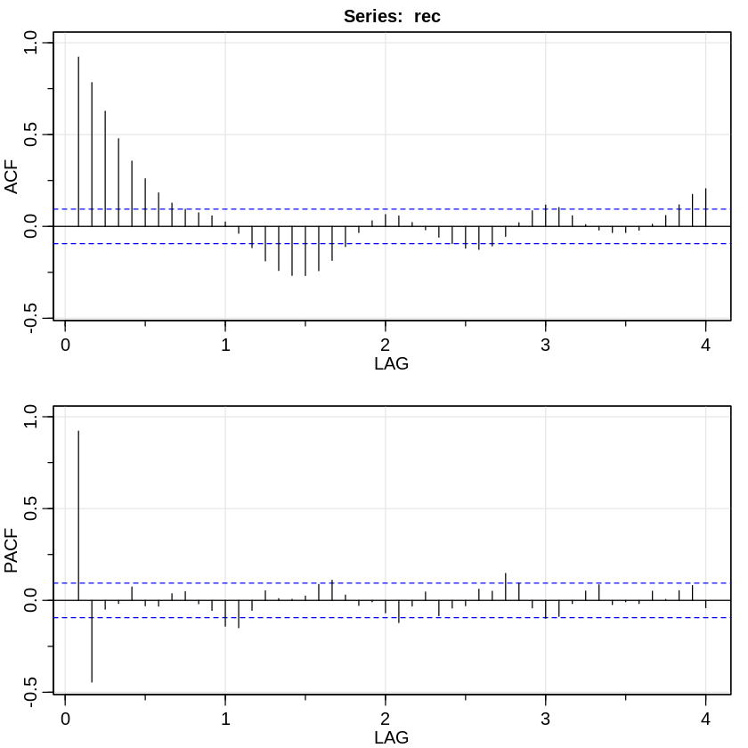
여기서 ACF의 graph에서 lag가 큰 경우, 이론적으론 0가 되어야하지만 실제론 그렇지 않다.
이것을 보정하기 위해 ACF값에 boundary([-$\frac{2}{\sqrt{n}}, \frac{2}{\sqrt{n}}$])를 잡고 이 안의 값은 95%의 확률로 0에 가깝다고 간주한다.
즉, 다음과 같은 가정을 한다.
$\hat \rho_X(h) \sim N(0, 1 / \sqrt{n}) \text{ for large } n$
최종적으로 lag = 1, 2 인 경우를 제외하곤 전부 0으로 간주하기 때문에 AR(2)가 적절하다는 결정을 내리게 된다.
2. Model building
- We need to decide $p, q$ in ARMA($p, q$)
- Estimate $\phi$s in ARMA($p, q$)
- Verify that it is a reasonable model
- Predict
이 중, 1~3 과정을 다음과 같이 나타내기도 한다.
- ACF and PACF
- For large $n$ cases, test if residual follows WN after fitting the model
1) Box-Ljung test
2) Sign test
3) Rank test
4) Q-Q plot - AIC, BIC, FPE: theoretical predictive power
- Cross Validation: empirical predictive power
1) Example: ARMA(p, q)
- From the $\rho(h)$’s viewpoint, $X_t \sim ARMA(p, q)$
⇒ Find residuals $\approx$ WN
- Testing
1) Test if ACF follows WN
\(\begin{cases} H_0: \hat \rho(h) \text{ is the same as that of WN} \\ H_a: \text{not } H_0 \end{cases} \\ \text{Recall that } \hat \rho_X(h) \sim N(0, 1 / n) \text{ for large } n \\ \text{Usually, we take the 95% CI of $\hat \rho(h)$ to be } 2 / \sqrt{n}\)
To understand it,
For white noise $a_1, \cdots, a_n$ ($E[a_t] = 0, Var(a_t) = 1$)
$\hat \rho(h) = \frac{1}{n-h} \sum_{t={h+1}}^n a_t a_{t-h}$
$E[\hat \rho(h)] = \frac{1}{n-h} \sum_{t={h+1}}^n E[a_t a_{t-h}] = 0$
$Var(\hat \rho(h)) = \frac{1}{(n-h)^2} Var(\sum_{t={h+1}}^n a_t a_{t-h}) = \frac{1}{n-h} \approx \frac{1}{n}$
2) Another way of testing $\hat a_t$ follows white noise is Ljung-Box-Pierce Q-statistics (kind of $\chi^2$ test)
If white noise,
\(\begin{aligned} \hat \gamma_h &\sim N(0, \frac{1}{n}) \\ \sqrt{n} \hat \gamma_h &\sim N(0, 1) \\ (\sqrt{n} \hat \gamma_h)^2 &\sim \chi_1^2 \\ (\sqrt{n} \hat \gamma_1)^2 + (\sqrt{n} \hat \gamma_2)^2 &\sim \chi_2^2 \\ \end{aligned}\)
Thus, Box-Pierce statistic for ARMA($p, q$)
$Q = n \sum_{h=1}^k \hat \gamma_h^2 \sim \chi_{k-p-q}^2$ ($k$는 대략 20 정도로 정한다)
만약, $Q$값이 크다면 해당 model을 기각할 수 있는 근거가 될 수 있다.
3) Another way is to construct a Q-Q plot of $\hat a_t$
Check if the residuals follow a normal distribution
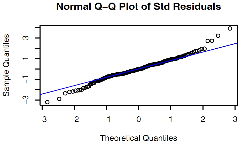
만약, $\hat a_t$가 normal dist.를 따른다면 Q-Q plot은 위와 같이 거의 직선에 근사한 graph가 된다.
Q-Q plot은 $\hat a_t$ 전체의 분포를 확인하는 것인 반면, Box-Pierce test는 각 $\hat a_t$ 간의 inter-relatedness를 확인하는 검정방법이라는 차이가 있다.
2) Deep into the AIC, BIC from ARMA(p, q)
\(\begin{aligned}
\text{AIC (Akaike Criterion)} &= -2 \log{\hat L} + \frac{2(p+q+1)n}{n-p-q-2} \\
&= Likelihood + Panelty \\
\hat L &= \text{likelihood after fitting the } ARMA(p, q)
\end{aligned}\)
AIC의 값이 더 작은 model이 좋은 ARMA model이다.
\(\begin{aligned}
\text{BIC (Bayesian Information Criterion)} &= -2 \log{\hat L} + 2(p+q+1) \log n \\
&= Likelihood + Panelty \\
\hat L &= \text{likelihood after fitting the } ARMA(p, q)
\end{aligned}\)
동일하게, BIC의 값이 더 작은 model이 좋은 ARMA model이다.
-
잘못된 항이 있을 수 있음 ↩