1. pytest
Code profiling에 앞서, 간단히 소요시간과 작동을 확인하기 위해 pytest를 사용한다.
실험할 script file과 함수의 이름 앞에 test_를 붙여야 제대로 동작하니 주의.
반복된 실험으로 구한 평균으로 $\pi$의 값을 추정하는 Monte-Carlo approximation을 예제 코드로 만들어보았다. plot()을 통해 예쁜 실험결과를 확인할 수 있다.
1
2
3
4
5
6
7
8
9
10
11
12
13
14
15
16
17
18
19
20
21
22
23
24
25
26
27
28
29
30
31
32
33
34
35
36
37
38
39
40
41
42
43
44
45
### test_mc_sampling.py

from dataclasses import dataclass
import numpy as np
import matplotlib.pyplot as plt
plt.rc('axes', unicode_minus=False)


@dataclass
class Point:
    x: "X coordinate"
    y: "Y coordinate"
def monte_carlo_approx(num_samples):
    ### 1. Data
    points        = np.array([Point(*np.random.uniform(-1, 1, 2)) for _ in range(num_samples)])
    idxs_inside   = np.array([idx for idx, point in enumerate(points) if point.x**2 + point.y**2 <= 1])
    points_inside = points[idxs_inside]

    ### 2. Plot
    plot(num_samples, points, points_inside)
def plot(num_samples, points, points_inside):
    ### 1. Generate figure
    fig, ax = plt.subplots(figsize=(10, 10))

    ### 2. Plot figures
    ax_rect, = ax.plot([point.x for point in points], [point.y for point in points], '.', markersize=0.01)
    ax_circle, = ax.plot([point.x for point in points_inside], [point.y for point in points_inside], '.', markersize=0.02)
    ax.add_artist(plt.Rectangle((-1, -1), 2, 2, fill=False, color=ax_rect.get_color()))
    ax.add_artist(plt.Circle((0, 0), 1, fill=False, color=ax_circle.get_color()))

    ### 3. Options
    ax.set_xlabel('x', fontsize=20)
    ax.set_ylabel('y', fontsize=20)
    ax.grid(alpha=0.5)
    ax.set_title(f"Monte-Carlo approximated pi = {len(points_inside) / len(points) * (2 * 2):.3f} (#samples: {num_samples})", fontsize=20)
    fig.show()


def test_main():
    num_samples = 2**18
    monte_carlo_approx(num_samples)


if __name__ == '__main__':
    test_main()
$ pip install pytest
$ pytest test_mc_sampling.py::test_main
============================================= test session starts =============================================
platform linux -- Python 3.7.6, pytest-6.2.4, py-1.10.0, pluggy-0.13.1
rootdir: /home/ydj/project/playground/prof
collected 1 item

test_mc_sampling.py .                                               [100%]

============================ 1 passed in 5.70s ============================
(rapids) root@titan:~/playground/prof# pytest test_mc_sampling.py::test_main
=========================== test session starts ===========================
platform linux -- Python 3.7.6, pytest-6.2.4, py-1.10.0, pluggy-0.13.1
rootdir: /home/ydj/project/playground/prof
collected 1 item

test_mc_sampling.py .                                               [100%]

============================ 1 passed in 6.65s ============================
2. Profiling
Python에서 가장 유명한 profile tool은 vprof인 것 같다.
$ pip install vprof
pip를 사용하여 간단히 설치하고 다음 명령어를 쳐서 http 서버를 통해 profiling 결과를 볼 수 있다.
$ vprof -c cmhp test_mc_sampling.py

// -H option으로 host를 직접 지정할 수 있음
$ vprof -c cmhp test_mc_sampling.py -H 0.0.0.0
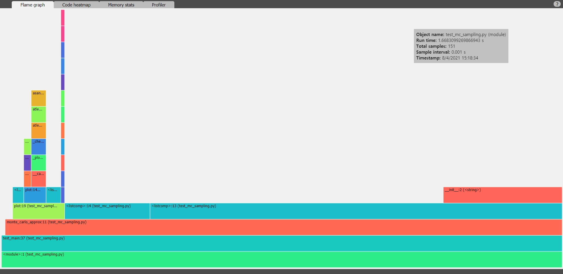
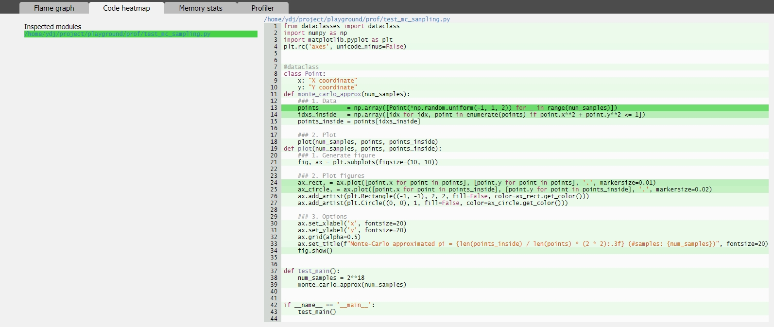
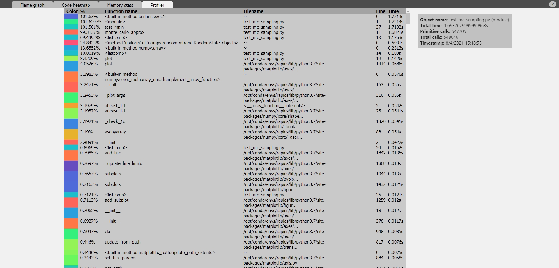
Memory stats 부분은 에러가 있는지 잘 안 나온다.. 나머지 부분들은 시각적으로 확실히 보기가 편하다.
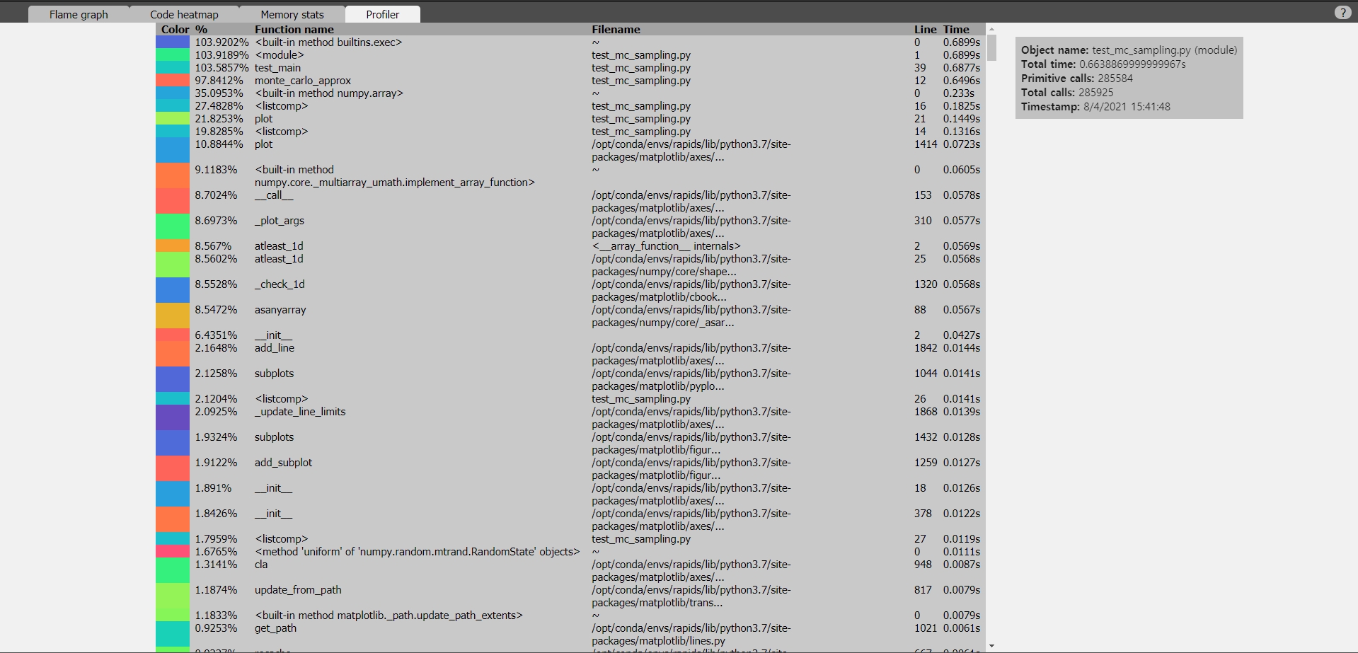
난수를 생성할 때 호출을 여러 번 해서 시간을 많이 잡아먹었는데, 이를 한 번만 호출하는 것으로 바꾸면 시간이 많이 단축된다.
1
2
points = np.array([Point(x, y) for x, y in zip(*np.random.uniform(-1, 1, (2, num_samples)))])
# points = np.array([Point(*np.random.uniform(-1, 1, 2)) for _ in range(num_samples)])
PREVIOUSEtc