Text Embedding

1. TF-IDF

여러 문서로 이루어진 문서군이 있을 때 어떤 단어가 특정 문서 내에서 얼마나 중요한 것인지를 나타내는 통계적 수치

TF(Term Frequency)
$tf(t, d)$ : 문서 $d$에서 단어 $t$의 등장 횟수

IDF(Inverse Document Frequency)
$df(t, D) = \mid {d \in D : t \in d } \mid$ : 문서 집합 $D$ 중 단어 $t$가 등장한 문서의 개수 $idf(t, D) = log \frac{|D|}{1+df(t, D)}$ : $df(t, D)$ 와 반비례하는 값

TF-IDF
$tfidf(t, d, D) = tf(t, d) \times idf(t, D)$ : 문서 집합 $D$에 속한 문서 $d$ 내에서 단어 $t$가 얼마나 중요한 지를 나타내는 통계적 수치

1) Pros & Cons

Pros
- 직관적인 해석이 가능
Cons
- 높은 차원을 가지는 sparse embedding으로 메모리 효율성이 낮음

2) Code

1
2
3
4
5
6
7
8
9
10
11
12
13
14
15
16
17
18
import pandas as pd
from sklearn.feature_extraction.text import TfidfVectorizer
import matplotlib.pyplot as plt

data = [
  '먹고 싶은 사과',
  '먹고 싶은 바나나',
  '길고 노란 바나나 바나나',
  '저는 과일이 좋아요'
]

enc = CountVectorizer()
emb = enc.fit_transform(data).toarray()
emb = pd.DataFrame(emb, columns=sorted(enc.vocabulary_))

print(f"(# documents, # terms) = {emb.shape}")
display(emb)
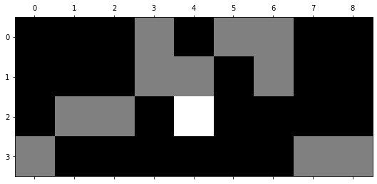
plt.matshow(emb, cmap='gray');

(# documents, # terms) = (4, 9)

        과일이	길고	노란	먹고	바나나	사과	싶은	저는	좋아요
0	0	0	0	1	0	1	1	0	0
1	0	0	0	1	1	0	1	0	0
2	0	1	1	0	2	0	0	0	0
3	1	0	0	0	0	0	0	1	1

tf-idf 1

1
2
3
4
5
6
7
8
9
10
11
12
13
14
15
16
17
18
import pandas as pd
from sklearn.feature_extraction.text import TfidfVectorizer
import matplotlib.pyplot as plt

data = [
  '먹고 싶은 사과',
  '먹고 싶은 바나나',
  '길고 노란 바나나 바나나',
  '저는 과일이 좋아요'
]

enc = TfidfVectorizer()
emb = enc.fit_transform(data).toarray()
emb = pd.DataFrame(emb, columns=sorted(enc.vocabulary_))

print(f"(# documents, # terms) = {emb.shape}")
display(emb)
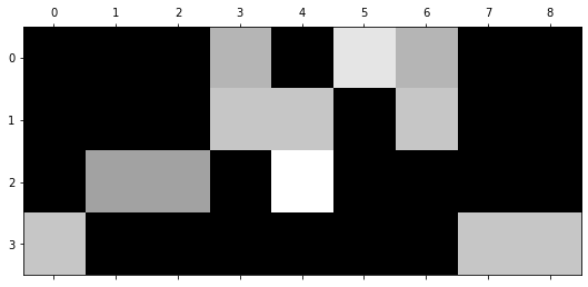
plt.matshow(emb, cmap='gray');

(# documents, # terms) = (4, 9)
        과일이	길고	노란	먹고	바나나	사과	싶은	저는	좋아요
0	0.00	0.00	0.00	0.53	0.00	0.67	0.53	0.00	0.00
1	0.00	0.00	0.00	0.58	0.58	0.00	0.58	0.00	0.00
2	0.00	0.47	0.47	0.00	0.74	0.00	0.00	0.00	0.00
3	0.58	0.00	0.00	0.00	0.00	0.00	0.00	0.58	0.58

tf-idf 2

1
2
3
4
5
6
7
8
9
10
11
12
import pandas as pd
from sklearn.feature_extraction.text import TfidfVectorizer
import matplotlib.pyplot as plt

data = pd.read_csv('movies_metadata.csv', low_memory=False).dropna()['overview']
enc = TfidfVectorizer(stop_words='english')
emb = enc.fit_transform(data).toarray()
emb = pd.DataFrame(emb, columns=sorted(enc.vocabulary_))

print(f"(# documents, # terms) = {emb.shape}")
display(emb)
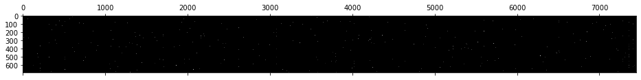
plt.matshow(emb, cmap='gray');

(# documents, # terms) = (4, 9)
        과일이	길고	노란	먹고	바나나	사과	싶은	저는	좋아요
0	0.00	0.00	0.00	0.53	0.00	0.67	0.53	0.00	0.00
1	0.00	0.00	0.00	0.58	0.58	0.00	0.58	0.00	0.00
2	0.00	0.47	0.47	0.00	0.74	0.00	0.00	0.00	0.00
3	0.58	0.00	0.00	0.00	0.00	0.00	0.00	0.58	0.58

tf-idf 3

2. Word2Vec

단어간 유사도를 반영하여 저차원 공간의 vector로 변환하는 방법

1) Algorithm

CBOW와 Skip-Gram 2가지 알고리즘을 사용할 수 있으며,
일반적으로 Skip-Gram의 성능이 더 좋은 것으로 알려져 있다.

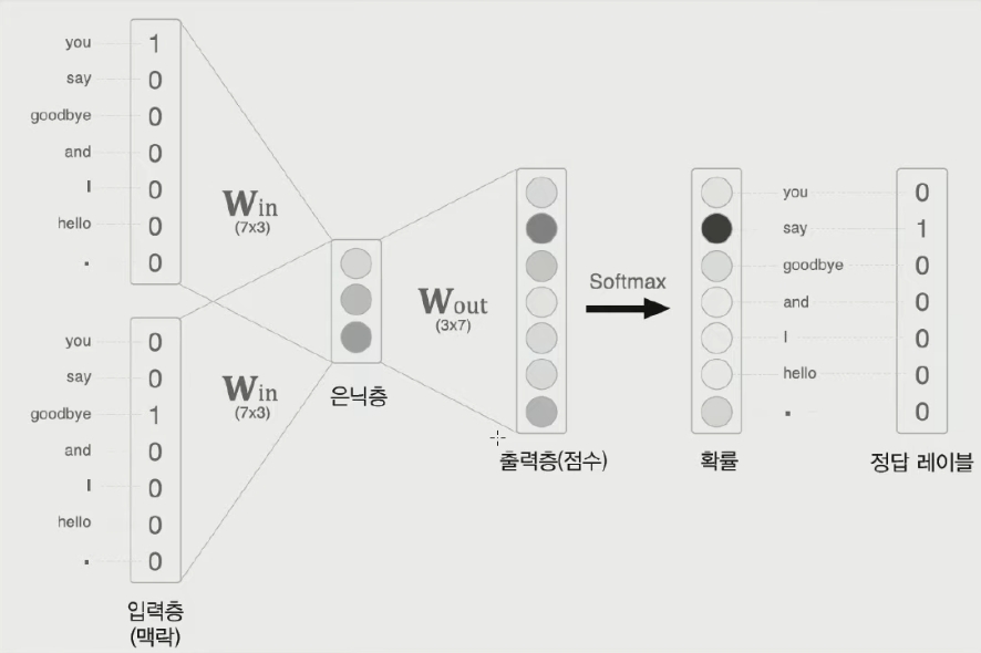
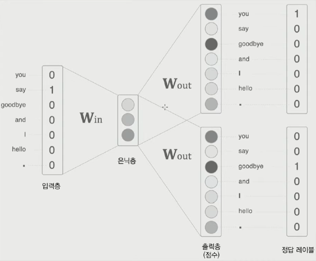
- CBOW

주변 단어들과 가운데 단어의 one-hot encoding을 각각 input과 output으로 하는 모델을 학습시키는 알고리즘


그림 1. 주변 단어를 보고 가운데 단어를 예측하는 CBOW 모델	그림 2. Supervised learning을 통해 학습되는 $W_{in}$ 을 embedding vector로 사용

- Skip-Gram

가운데 단어와 주변 단어들의 one-hot encoding을 각각 input과 output으로 하는 모델을 학습시키는 알고리즘


그림 1. 가운데 단어를 보고 주변 단어들을 예측하는 Skip-Gram 모델	그림 2. Supervised learning을 통해 학습되는 $W_{in}$ 을 embedding vector로 사용

2) Pros & Cons

Pros
- Dimension을 임의로 정해줄 수 있는 dense embedding 방법으로 메모리 효율성이 높음
- ANN을 사용하기 때문에 GPU를 활용한 병렬처리가 가능함
- 학습을 통해 모델의 개선이 가능

3) Code

1
2
3
4
5
6
7
8
9
10
11
12
13
14
15
16
17
18
19
import pandas as pd
import gensim
from gensim.models import Word2Vec
from nltk.tokenize import word_tokenize
import matplotlib.pyplot as plt

data = pd.read_csv('movies_metadata.csv', low_memory=False)['overview'].dropna().values
sentence = list(map(word_tokenize, data))
emb_model = Word2Vec(sentence,
                     vector_size=20,  # dimension of embedding vector
                     window=5,        # maximum distance between the input, output word
                     min_count=1,     # ignore all words with frequency lower than this
                     sg=1,            # 1: skip-gram, 0: CBOW
                     epochs=500,
                     workers=-1)

print("- Length of sentence:", len(sentence))
print(sentence[0])
emb_model.wv.most_similar('beautiful')

- Length of sentence: 44512
['Led', 'by', 'Woody', ',', 'Andy', "'s", 'toys', 'live', 'happily', 'in', 'his', 'room', 'until', 'Andy', "'s", 'birthday', 'brings', 'Buzz', 'Lightyear', 'onto', 'the', 'scene', '.', 'Afraid', 'of', 'losing', 'his', 'place', 'in', 'Andy', "'s", 'heart', ',', 'Woody', 'plots', 'against', 'Buzz', '.', 'But', 'when', 'circumstances', 'separate', 'Buzz', 'and', 'Woody', 'from', 'their', 'owner', ',', 'the', 'duo', 'eventually', 'learns', 'to', 'put', 'aside', 'their', 'differences', '.']

[('Counts', 0.781749963760376),
 ('Muktada', 0.777137279510498),
 ('Carras', 0.7720910310745239),
 ('-Luke', 0.7681071162223816),
 ('Mascarenas', 0.7541091442108154),
 ('Fúsi', 0.7538864016532898),
 ('troubadour', 0.7512907981872559),
 ('Whelen', 0.7433350086212158),
 ('Heineken', 0.7424498200416565),
 ('con', 0.7377300262451172)]

Pretrained model

1
2
3
4
5
import gensim.downloader

# model = gensim.downloader.load('wiki-english-20171001')  # heavy
model = gensim.downloader.load('glove-twitter-25')  # light
model.most_similar('beautiful')

[('gorgeous', 0.9333646297454834),
 ('lovely', 0.9279096722602844),
 ('amazing', 0.9218392968177795),
 ('love', 0.9173234105110168),
 ('wonderful', 0.9150214195251465),
 ('loving', 0.9093379974365234),
 ('dream', 0.9086582660675049),
 ('pretty', 0.907191276550293),
 ('perfect', 0.9066721796989441),
 ('little', 0.9064547419548035)]

3. Doc2Vec

문서간 유사도를 반영하여 저차원 공간의 vector로 변환하는 방법

1) Code

1
2
3
4
5
6
7
8
9
10
11
12
13
14
15
16
17
18
19
20
21
22
23
24
25
26
27
28
29
30
31
32
import re
from tqdm import tqdm

import pandas as pd
from gensim.models import doc2vec
from gensim.models.doc2vec import TaggedDocument
from nltk.corpus import stopwords
from nltk.tokenize import word_tokenize

# Data: https://www.kaggle.com/code/chocozzz/00-word2vec-1/data?select=movies
meta = pd.read_csv('movies_metadata.csv', low_memory=False)
meta = meta[meta['original_title'].notnull()].reset_index(drop=True)
meta = meta[meta['overview'].notnull()].reset_index(drop=True)

overview = []
for sentence in tqdm(meta['overview']):
    sentence = re.sub('[^A-Za-z0-9]+', ' ', sentence).strip().lower()
    tokens   = word_tokenize(sentence)
    overview.append([word for word in tokens if word not in set(stopwords.words('english'))])
meta['pre_overview'] = overview
tagged_corpus = [TaggedDocument(words, [tag]) for words, tag in meta[['pre_overview', 'original_title']].values]


sample = meta.iloc[0]
print("1. Original title")
print(sample['original_title'], '\n')

print("2. Overview")
print(sample['overview'], '\n')

print("3. Tagged corpus")
print(tagged_corpus[0])

1. Original title
Toy Story

2. Overview
Led by Woody, Andy's toys live happily in his room until Andy's birthday brings Buzz Lightyear onto the scene. Afraid of losing his place in Andy's heart, Woody plots against Buzz. But when circumstances separate Buzz and Woody from their owner, the duo eventually learns to put aside their differences.

3. Tagged corpus
TaggedDocument<['led', 'woody', 'andy', 'toys', 'live', 'happily', 'room', 'andy', 'birthday', 'brings', 'buzz', 'lightyear', 'onto', 'scene', 'afraid', 'losing', 'place', 'andy', 'heart', 'woody', 'plots', 'buzz', 'circumstances', 'separate', 'buzz', 'woody', 'owner', 'duo', 'eventually', 'learns', 'put', 'aside', 'differences'], ['Toy Story']>

1
2
3
4
5
6
7
8
9
10
11
12
13
14
15
16
doc_vectorizer = doc2vec.Doc2Vec(
    dm=0,          # PV-DBOW / default=1
    dbow_words=1,  # w2v simultaneous with DBOW d2v / default=0
    window=10,     # distance between the predicted word and context words
    vector_size=100,
    alpha=0.025,
    min_count=5,
    min_alpha=0.025,
    workers=-1,
    hs=1,
    negative=10
)
doc_vectorizer.build_vocab(tagged_corpus)
print(f"Tag Size: {len(doc_vectorizer.dv.key_to_index)}")
doc_vectorizer.train(tagged_corpus, total_examples=doc_vectorizer.corpus_count, epochs=doc_vectorizer.epochs)
doc_vectorizer.dv.most_similar('Toy Story')

Tag Size: 42446
CPU times: user 1.67 s, sys: 43.6 ms, total: 1.71 s
Wall time: 1.7 s
[('Armaguedon', 0.4034751355648041),
 ('Ali Baba Bunny', 0.4009561240673065),
 ('These Girls', 0.3865448236465454),
 ('காதல் கோட்டை', 0.3724530041217804),
 ('American Sharia', 0.3583838939666748),
 ('Dumbland', 0.35733845829963684),
 ('Honeymoon in Bali', 0.3508087694644928),
 ('A Field in England', 0.34832653403282166),
 ('IMAX Mummies Secrets Of The Pharohs', 0.33970147371292114),
 ('ラビット・ホラー３Ｄ', 0.33751049637794495)]

Reference

PREVIOUSEtc