1. Introduction
데이터에서 가장 분산이 큰 축을 찾아 투영시키는 방법
데이터와 투영된 것 사이의 MSE(reconstruction error)를 최소화하는 축을 찾는 방법으로도 생각할 수 있다.
2. Background
2.1 Information
정보를 많이 가지고 있다는 것은 다양성(불확실성)이 크다는 것이다.
즉, 데이터의 분산이 클수록 많은 정보를 가지는 것으로 이해할 수 있다.
자세한 내용은 Information theory를 참고
2.2 Eigenvalue, eigenvector
Square matrix $A$에 대하여 $A \mathbf x = \lambda \mathbf x \ (\mathbf x \neq \mathbf 0)$를 만족시키는 vector $\mathbf x$를 eigenvector, $\lambda$를 eigenvalue라 한다.
이는, linear transformation($A$)이 일어난 후에도 방향이 변하지 않고 세기($\lambda$)만 변하는 vector($\mathbf x$)를 나타낸다.
자세한 내용은 Eigenvalue and eigenvector를 참고
2.3 Eigenvalue/spectral decomposition
- Regular matrix $A(n \times n)$는 $n$개의 eigenvalue와 linearly independent eigenvector를 가진다.
- $(A - \lambda I) \mathbf x = \mathbf 0 \ (\mathbf x \neq \mathbf 0)$
- $det(A - \lambda I) = 0$
- $n$차 방정식의 해(eigenvalue)는 $n$개 존재
- Eigenvalue decomposition
\(\begin{equation} \begin{aligned} A \begin{bmatrix} \\ \mathbf{p}_1 & \cdots & \mathbf{p}_n \\ \\ \end{bmatrix} &= \begin{bmatrix} \\ \mathbf{p}_1 & \cdots & \mathbf{p}_n \\ \\ \end{bmatrix} \begin{bmatrix} \lambda_1 & \cdots & 0\\ \vdots & \ddots & \vdots\\ 0 & \cdots & \lambda_n\\ \end{bmatrix} \\ AP &= P \Lambda \\ \therefore \ A &= P \Lambda P^{-1} \end{aligned} \\ \end{equation}\) - Spectral decomposition
만약 $A$가 symmetric이면, $P$가 orthogonal matrix가 되어 $P^{-1} = P’$ 가 성립
$\therefore \ A = P \Lambda P’$
3. Algorithm
- Notation
\(X: \text{original data} \ (n, d) \quad (n: \text{number of data}, \ d: \text{dimension of data}) \\ X = \begin{bmatrix} \\ \mathbf{x}_1 & \cdots & \mathbf{x}_d \\ \\ \end{bmatrix} \quad \cdots \quad \text{Shift mean for all column vector: } \ \forall i \big( \frac{1}{n} \sum_j x_{ij} = 0 \big) \\ \quad \\ Z: \text{reduced(projected) data} \ (n, k) \quad (k: \text{reduced dimension}, \ k < d) \\ Z = \begin{bmatrix} \\ \mathbf{z}_1 & \cdots & \mathbf{z}_k \\ \\ \end{bmatrix} \\ \mathbf{z}_{i}: \text{score vector of the i'th principal component} \\ z_{ij}: \text{scores of the i'th principal component} \\ \quad \\ \Phi: \text{projection matrix} \ (d, k) \\ \Phi = \begin{bmatrix} \\ \mathbf{\phi}_1 & \cdots & \mathbf{\phi}_k \\ \\ \end{bmatrix} \\ \mathbf{\phi}_i: \text{loading vector of the i'th principal component} \\ \phi_{ij}: \text{loadings of the i'th principal component} \\\)
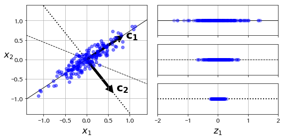
- PCA는 linear transformation(projection)을 통해 차원을 축소한다.
- 투영된 데이터가 정보를 가장 많이 가지고 있는(분산이 가장 큰) 축(principal component)을 선택한다.
- 첫 번째 축에 투영된 데이터($\mathbf{z}_1$)는 다음과 같이 표현이 가능하다.
\(\mathbf{z}_1 = X \mathbf{\phi}_1 = \phi_{11} \mathbf{x}_1 + \cdots + \phi_{d1} \mathbf{x}_d \\ \begin{bmatrix} \\ \mathbf{z}_1 \\ \\ \end{bmatrix} = \begin{bmatrix} \\ \mathbf{x}_1 & \cdots & \mathbf{x}_d \\ \\ \end{bmatrix} \begin{bmatrix} \\ \mathbf{\phi}_1 \\ \\ \end{bmatrix} \quad \cdots \quad \text{Contraint for comparating variances: } || \mathbf{\phi}_1 ||^2 = 1 \\\) - $\mathbf{z}_1$의 분산을 최대화시키는 $\mathbf{\phi}_1$을 선택한다.
\(Var(\mathbf{z}_1) = \frac{1}{n} \mathbf{z}_1' \mathbf{z}_1 \quad \cdots \quad \text{ mean}(\mathbf{x}_1) = \text{ mean}(\mathbf{z}_1) = \mathbf{0} \\ \quad \\ \begin{equation} \begin{aligned} \hat{\mathbf{\phi}}_1 &= argmax_{\mathbf{\phi}_1} Var(\mathbf{z}_1) \\ \hat{\mathbf{\phi}}_1 &= argmax_{\mathbf{\phi}_1} \big( \mathbf{\phi}_1' X'X \mathbf{\phi}_1 \big) \\ &= argmax_{\mathbf{\phi}_1} \big( \mathbf{\phi}_1' P \Lambda P' \mathbf{\phi}_1 \big) \quad \cdots \quad \text{Spectral decomposition} \\ &= argmax_{\mathbf{\phi}_1} \big( \mathbf{\alpha}' \Lambda \mathbf{\alpha} \big) \quad \cdots \quad \alpha \equiv P' \mathbf{\phi} \ (\text{orthogonal transformation}) \\ &= argmax_{\mathbf{\phi}_1} \big( \lambda_1 \alpha_1^2 + \cdots + \lambda_d \alpha_d^2 \big) \quad \quad s.t. \ ||\alpha||^2 = 1, \ \lambda_1 > \lambda_2 > \cdots > \lambda_d \\ \end{aligned} \end{equation} \\ \hat{\mathbf{\alpha}} = [1, 0, \cdots, 0]' \\ \quad \\ \max_{\mathbf{\phi}_1}Var(\mathbf{z}_1) = \lambda_1 \\ \hat{\mathbf{\phi}}_1 = \mathbf{p}_1 \\\) - $\mathbf{z}_2$의 분산을 최대화시키는 $\mathbf{\phi}_2$을 선택한다.
단, 중복된 정보를 배제하기 위하여 선택된 principal components($\mathbf{\phi}_1$)와 orthogonal한 축을 선택한다. \(\begin{equation} \begin{aligned} \hat{\mathbf{\phi}}_2 &= argmax_{\mathbf{\phi}_2} Var(\mathbf{z}_2) \\ &\quad \quad \quad \vdots \\ &= argmax_{\mathbf{\phi}_2} \big( \lambda_1 \alpha_1^2 + \cdots + \lambda_d \alpha_d^2 \big) \quad \quad s.t. \ ||\alpha||^2 = 1, \ \lambda_1 > \lambda_2 > \cdots > \lambda_d \\ &= argmax_{\mathbf{\phi}_2} \big( \lambda_2 \alpha_2^2 + \cdots + \lambda_d \alpha_d^2 \big) \quad \cdots \quad \alpha_1 = \mathbf{p}_1' \mathbf{\phi}_2 = \mathbf{0} \ (\text{orthogonal constraint})\\ \end{aligned} \end{equation} \\ \hat{\mathbf{\alpha}} = [0, 1, \cdots, 0]' \\ \quad \\ \max_{\mathbf{\phi}_2}Var(\mathbf{z}_2) = \lambda_2 \\ \hat{\mathbf{\phi}}_2 = \mathbf{p}_2 \\\) - 반복하여, $\mathbf{z}_k$의 분산을 최대화시키는 $\mathbf{\phi}_k$까지 선택한다. \(\hat{\mathbf{\phi}}_k = \mathbf{p}_k \\\)
- 첫 번째 축에 투영된 데이터($\mathbf{z}_1$)는 다음과 같이 표현이 가능하다.
- Score matrix $Z$는 다음과 같은 projection을 통해 투영된 것으로 나타낼 수 있다. \(\begin{equation} \begin{aligned} Z &= X \Phi \\ \begin{bmatrix} \\ \mathbf{z}_1 & \cdots & \mathbf{z}_k \\ \\ \end{bmatrix} &= \begin{bmatrix} \\ \mathbf{x}_1 & \cdots & \mathbf{x}_d \\ \\ \end{bmatrix} \begin{bmatrix} \\ \mathbf{p}_1 & \cdots & \mathbf{p}_k \\ \\ \end{bmatrix} \end{aligned} \end{equation}\)
4. Kernel PCA
비선형 subspace로 투영하는 PCA
- 투영된 후에도 cluster를 유지하거나, manifold에 가까운 데이터를 펼칠 때에 유용하다.
5. Hyperparameter tuning
Unsupervised learning이므로 score를 직접 지정할 필요가 있다.
- Problem-specific score
- Reconstruction error
- Pre-image error
- Reconstruction이 불가능한 경우, mapping을 학습($f: Y → X$)하여 pre-image(원상)을 추정
6. Code
- Parameters
n_components: int(PC의 개수) or float(explained variance ratio),mlesvd_solver:auto(randomorfull, default),randomized(fast randomized SVD),full(exact full SVD)
- Time complexity
full: $O(d^3 + d^2 n)$randomized: $O(k^3 + k^2 n) (k: \text{n_components})$
1
2
3
4
5
6
7
8
9
10
11
12
13
14
import numpy as np
from sklearn.decomposition import PCA, KernelPCA

X = np.array([[-1, -1], [-2, -1], [-3, -2], [1, 1], [2, 1], [3, 2]])

pca = PCA(n_components=2, svd_solver='full').fit(X)
X_red = pca.transform(X)
X_rec = pca.inverse_transform(X_red)  # reconstruction error: mse(X, X_rec)
print(pca.explained_variance_ratio_)
print(pca.singular_values_)

kpca = KernelPCA(n_components=2, kernel='rbf', gamma=0.04, fit_inverse_transform=True).fit(X)
X_red = kpca.transform(X)
X_pre = kpca.inverse_tran+sform(X_red)  # pre-image
PREVIOUSEtc