Remarks
120. Graph Neural Network(GNN)의 정의부터 응용까지 (한국원자력연구원 인공지능응용전략실 최희선 선임연구원), [논문 리뷰] Graph Neural Networks (GCN, GraphSAGE, GAT) - 김보민 등의 내용을 정리한 글입니다.
1. Introduction to Graph Neural Networks
1.1 Graph representation learning
Graph representation learning
Summarizing the structure of a graph in a low dimensional space(embedding space)
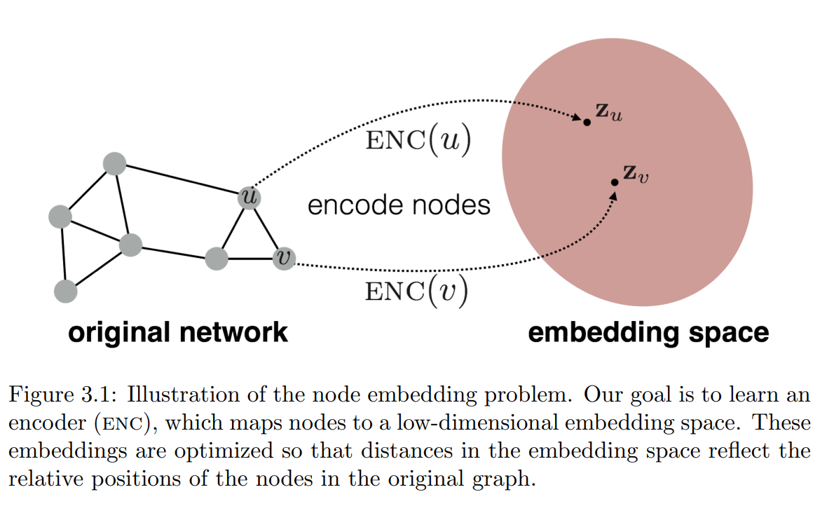
1.2 Node embedding
1.2.1 Shallow embedding method
General embedding like NLP
- One-hot encoding nodes
- Embed with matrix (embedder, shape: [#emb_dim, #nodes])
- How to learning embedder
- Measure smilarity between nodes: $S(A, C)$
- Optimize the parameters of the embedder to preserve the similarity
$S(A, C) \approx S(E(A), E(C))$
- Inherent issues
- The size of an embedder increases linearly with the number of nodes
- Difficult in defining the similarity metric
- Example
Node2Vec, DeepWalk, LINE, …- Node2Vec performs good if don’t matter the embedder size
1.2.2 Neural network-based methods
- Message passing GNN
- Concept: a node is represented with the neighbors(context)
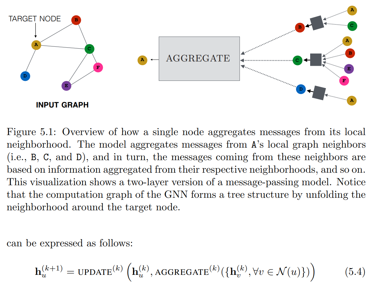
- UPDATE, AGGREGATE: arbitrary differentiable functions (e.g. NN)
- Weisfeiler-Lehman GNNs
pass
1.3 Notation
Given a graph $G$:
- $V$: set of vertices
- $A$: binary adjacency matrix
- $X \in R^{m \times \mid V \mid}$: a matrix of node features
1.4 Graph tasks
- Node classification
Categorize users/items - Link prediction
Grpah completion - Graph classification
Molecule property prediction - Clustering
Social circle detection - Graph generation
Drug discovery
2. Graph Convolution Networks (GCN, ICLR 2017)
2.1 CNN vs GCN
- CNN: Spatial location(euclidean distance) based
- GCN: Neighborhood(edge) based
2.2 Concept
Theoretical point of view: “Neighborhood Normalization”
- Aggregation without normalization (previous)
$\sum_{v \in \mathcal{N}(u)} h_v$: unstable and highly sensitive to node degrees - Use symmetric normalization aggregation function (proposed)
$\sum_{v \in \mathcal{N}(u)} h_v \rarr \sum_{v \in \mathcal{N}(u)} \frac{h_v}{\sqrt{ \mid \mathcal{N}(u) \mid \mid \mathcal{N}(v) \mid }}$
2.3 Learning node embeddings: iterative method
2.3.1 GCN layer
$H^{(l+1)} = \sigma(\tilde D^{-1/2} \tilde A \tilde D^{-1/2} \ H^{(l)} W^{(l)})$
$H^{(l+1)} = \sigma(\quad \quad \ \ \hat A \ \ \ \quad\quad H^{(l)} W^{(l)})$
$\sigma: \text{ReLU}$
- $H^{(l)} \in R^{N \times D}$: matrix of activations in the $l$-th layer
- $\tilde A = A + I_N$: adjacency matrix + self-connections
$\tilde D_{ii} = \sum_j \tilde A_{ij}$: diagonal matrix - $\hat A = \tilde D^{-1/2} \tilde A \tilde D^{-1/2}$: normalized adjacency matrix (preprocessing)
Smaller degree${i}$ → bigger $A’{ii}$ - $H^{(0)} = X$
- $\hat A H^{(l)}$: aggregation(linear combination of node feature2)
$i$-th row: weighted sum of adjacent node features of $i$-th node
ex) 2-layer GCN (classification)
- Preprocessing
$\hat A = \tilde D^{-1/2} \tilde A \tilde D^{-1/2}$ - Forward
$Z_1 \ \ = \quad \quad \quad \quad \text{ReLU} (\hat A X W^{(0)})$
$Z_{out} = \text{softmax}(\text{ReLU} (\hat A Z_1 W^{(1)}))$ - Loss function(CEE)
$L = \sum_l \sum_f y_{lf} \ln Z_{lf}$
2.4 Key factors
- Definition of neighborhood
- Distance
- Adjacency matrix
- How to aggregate
- Attention and Edge weights
- (Neighborhood) Normalization
- Ordering of nodes (cf. check permutation invariance / equivalence)
2.5 Deep Graph Library(DGL)
DEEP GRAPH LIBRARY: Easy Deep Learning on Graphs
from torch import nn
import torch.nn.functional as F
from dgl.nn import GraphConv


class GCN(nn.Module):
    def __init__(self, in_feats, h_feats, num_classes):
        super(GCN, self).__init__()
        self.conv1 = GraphConv(in_feats, h_feats)
        self.conv2 = GraphConv(h_feats, num_classes)

    def forward(self, g, in_feat):
        h = self.conv1(g, in_feat)
        h = F.relu(h)
        h = self.conv2(g, h)
        return h
3. GraphSAGE (NeurIPS 2017)
3.1 GCN → GraphSAGE
- GraphSAGE
Generating embeddings by SAmpling and AGgregating features from a node’s local neighborhood
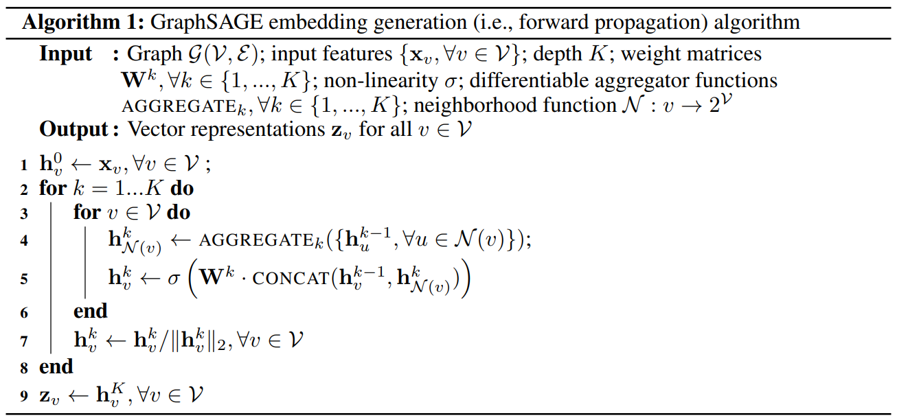
AGGREGATE- GraphSAGE-GCN: $\text{AGGREGATE}$ = weighted sum
- GraphSAGE-mean: $\text{AGGREGATE}$ = mean
- GraphSAGE-LSTM: $\text{AGGREGATE}$ = LSTM (high cost but not good)
- GraphSAGE-pool: $\text{AGGREGATE}$ = pool
3.2 Deep Graph Library(DGL)
from torch import nn
import torch.nn.functional as F
from dgl.nn import SAGEConv


class GCN(nn.Module):
    def __init__(self, in_feats, h_feats, num_classes):
        super(GCN, self).__init__()
        self.conv1 = SAGEConv(in_feats, h_feats, 'mean')
        self.conv2 = SAGEConv(h_feats, num_classes, 'mean')

    def forward(self, g, in_feat):
        h = self.conv1(g, in_feat)
        h = F.relu(h)
        h = self.conv2(g, h)
        return h
4. Graph Attention Networks (GAT, ICLR 2018)
Veličković, Petar, et al. “Graph attention networks.” arXiv preprint arXiv:1710.10903 (2017).
4.1 GNN applied Attention
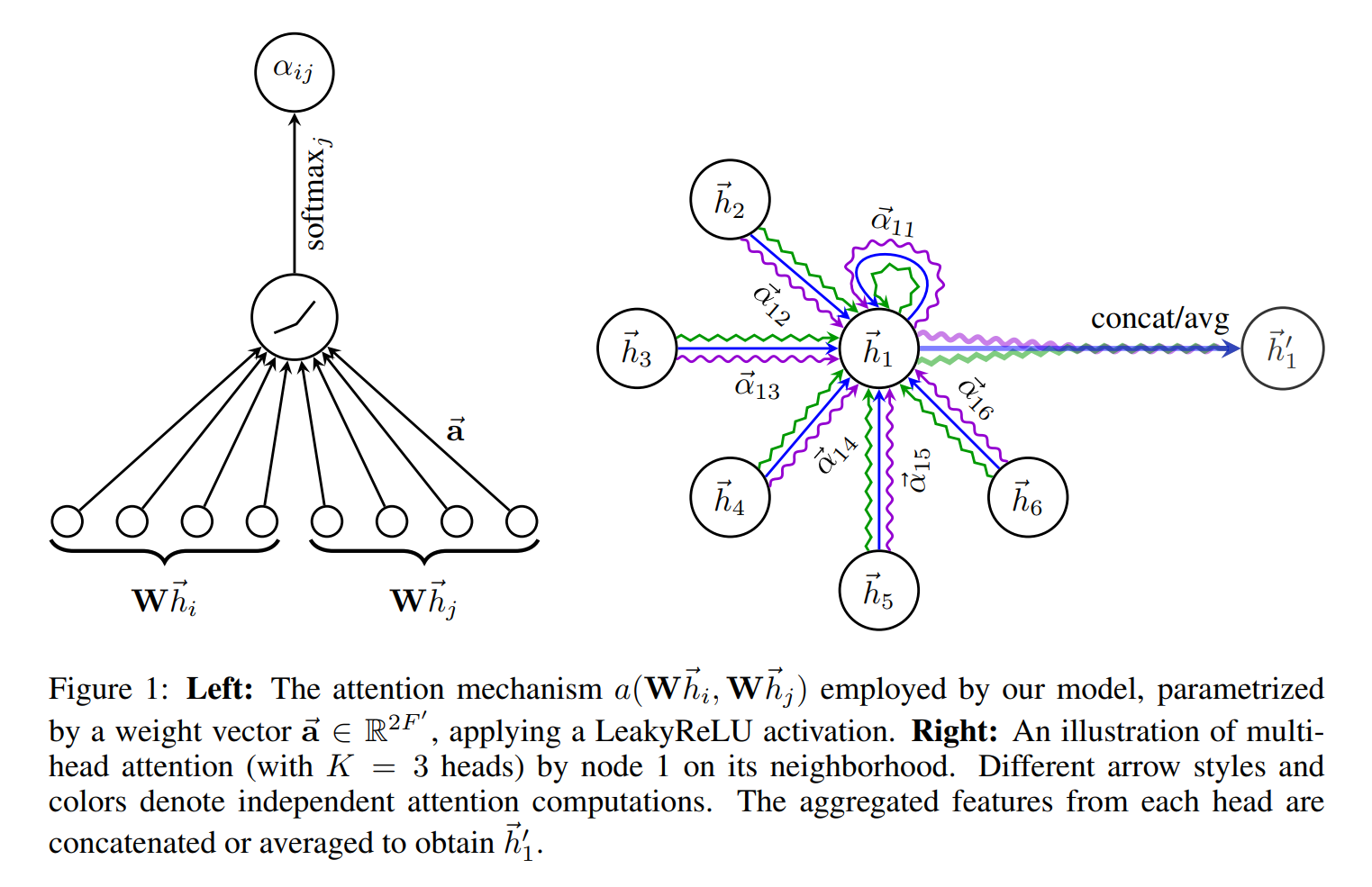
- Attention components
- Query: $h_j \in R^{F}$
- Key, value: $h_i \in R^{F}$
- Masked if not neighbors of $j$’th node
- Projection matrix: $W \in R^{F’ \times F}$
- Attention algorithm
- Transform input features($F$) into high-level features($F’$)
- Query: $h_j \rarr Wh_j$
- Key: $h_i \rarr Wh_i$
- Compute attention coefficients
- Attention mechanism $a: R^{2F’} \rarr R$
- Single-layer FC with LeakyReLU - $2F’$: concatenated query($F’$) and key($F’$)
- Compute attention coefficient
$e_{ij} = a(Wh_i, Wh_j)$
- Attention mechanism $a: R^{2F’} \rarr R$
- Normalize attention coefficient
$\alpha_{ij} = \text{softmax}j(e{ij})$ - Compute a linear combination of the features
$h’_i = \sigma(\sum_j \alpha_j Wh_j)$ -
Employ multi-head attention to stabilize the learning process
$h’^k_i = \sigma(\sum_j \alpha^k_j W^kh_j)$
$h’_i = \text{concat}_k(h’^k_i)$- On final(prediction) layer
$h’_i = \sigma(\text{mean}_k(\sum_j \alpha^k_j W^kh_j))$- Employ averaging instead of concatenation
- Delay applying nonlinarity
- On final(prediction) layer
- Transform input features($F$) into high-level features($F’$)
4.2 Deep Graph Library(DGL)
from torch import nn
import torch.nn.functional as F
from dgl.nn import GATConv


class GAT(nn.Module):
    def __init__(self, insize, hid_size, out_size, heads):
        super().__init__()
        self.conv1 = GATConv(in_size, hid_size, heads[0], feat_drop=0.6, attn_drop=0.6, activation=F.elu)
        self.conv2 = GATConv(hid_size*heads[0], out_size, heads[1], feat_drop=0.6, attn_drop=0.6, activation=None)

    def forward(self, g, inputs):
        h = self.conv1(g, inputs)
		h = h.flatten(1)
        h = self.conv2(g, h)
		h = h.mean(1)
        return h
References
- 120. Graph Neural Network(GNN)의 정의부터 응용까지 (한국원자력연구원 인공지능응용전략실 최희선 선임연구원)
- [논문 리뷰] Graph Neural Networks (GCN, GraphSAGE, GAT) - 김보민
- Kipf, Thomas N., and Max Welling. “Semi-supervised classification with graph convolutional networks.” arXiv preprint arXiv:1609.02907 (2016).
- Hamilton, Will, Zhitao Ying, and Jure Leskovec. “Inductive representation learning on large graphs.” Advances in neural information processing systems 30 (2017).
- Veličković, Petar, et al. “Graph attention networks.” arXiv preprint arXiv:1710.10903 (2017).